

回路で見る“ウェット”な電気化学と“ドライ”な電気化学
We just had our first laboratory in the advanced electrochemistry course that I teach this semester, and before starting “wet” electrochemistry in solution, I wanted to do a quick demonstration of the basic electrochemistry experiments using a so-called “equivalent circuit” (“equivalent cell”). I find that it is a nice way to show some of the concepts (and for us, it is also useful to troubleshoot any technical problems with the potentiostat). You could say it is a useless experiment, but it is also a nice way to look at how electrochemistry in solution can be modeled to a certain extent by using a simple circuit. Read more...
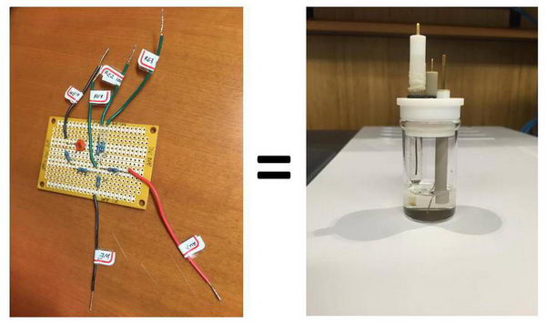
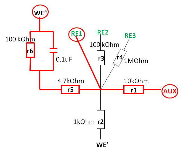
The equivalent circuit that I have made looks like this and it allows for various combinations:
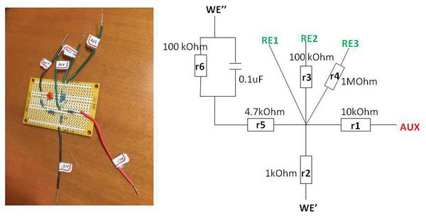
The green wires are modeling “reference electrodes” of different resistance: simple wire (RE1), 100 kOhm (RE2) and 1 MOhm (RE3). The red wire (AUX) is an “auxiliary electrode”, and 10 kOhm resistor (“r1”) attached there will be modeling compensated solution resistance. For working electrodes, we have several options – one without capacitor, (WE’), and one with capacitor (WE’’) as I will describe below. There is a resistor “r5” that models uncompensated solution resistance of electrochemical cell Ruc, and a capacitor (0.1 uF capacitance) (in parallel with r6) that will resemble electrical double layer capacitance in CV of the solution (typical values for capacitance 10-40 uF/cm2).
1. First, let’s start with simplest case and connect it as follows, through WE', RE1, and AUX:
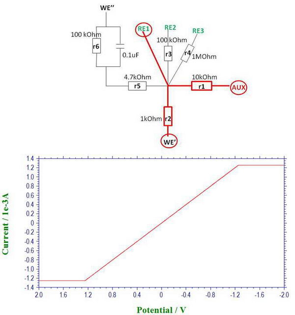
Then we can say that we try to model the conditions for electrolysis, since the current will be around 1 mA at 1V, which resembles a typical electrolysis experiment under our conditions. When we linearly scan the potential in a wide enough range, we can see two regions: one is a straight line that is follows Ohm’s law with slope depending on resistance “r2” (voltage 1V, current 1 mA, corresponding to “r2” of 1 kOhm). But when the potential difference is very high, we start seeing two flat regions which result from the limitations imposed by the compliance voltage of the potentiostat (the potential difference reaches the compliance voltage limit and it cannot increase anymore, so it stays constant).
In solution, you can sometimes encounter such limitations when doing electrolysis at low temperature or in high resistance solvent. For example, if you do low temperature electrolysis in THF solution at a relatively high potential, you are very likely to reach the limit of compliance voltage and the actual electrode potential will be lower than expected (and, of course, the electrolysis will slow down and it may not go to completion, depending on the system and reversibility).
2. The reason why we made a circuit with different resistant RE’s is to check how sensitive it becomes to electrical noise when using higher resistance RE. In solution, such high resistance reference may be the case when the membrane is damaged, or when non-aqueous membrane-separated Ag/AgNO3 in TBAP-MeCN reference is used at low temperature.
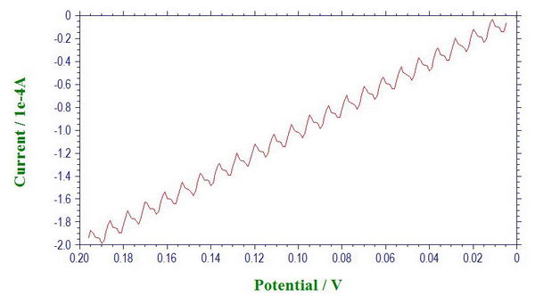
For example, connect the circuit though WE’, AUX and RE3 (connected through 1 MOhm resistor). We don’t use Faraday cage in this test. First, we see that the line starts becoming slightly more wavy than before (at 500 mV/s).
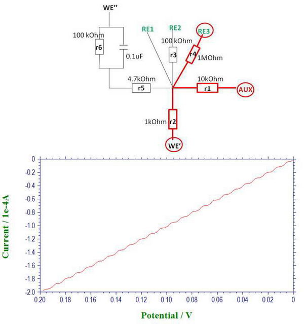
We can make it more pronounced by simply putting different electrical appliances in proximity to the circuit.
Here is what it looks like when we put it next to laptop AC adapter. We can see the noise originating from 60 Hz and also from 120 Hz (which is to be expected from bridge rectifier when converting AC to DC). (The noise frequencies are determined through Fourier transform as described in one of the previous posts.)
So that is actually a good reason to use Faraday cage in a lab full of electrical appliances, especially if you operate under high resistance conditions when picking up noise becomes much more of a problem, or when the current is very small (for example, with microelectrodes). It is sometimes easy to mistakenly interpret electrical noise as a real signal. So it is quite useful to perform this check with the equivalent circuit as the first step for any troubleshooting in the system or when moving the potenstiostat to work in a new environment.
3. Next, we want to model the electrical double layer, so we need to add a capacitor to the scheme. In addition, we have a resistor “r5” (4.7 kOhm) which models uncompensated “solution” resistance Ruc between working and reference electrodes.
The reason for choosing a 100 kOhm resistor for r6 is to give currents that are more typical for a CV experiment, in microampere range.
First thing we notice is the appearance of a “gap” between forward and reverse scans when we perform a basic cyclic voltammetry experiment. The size of this “gap” increases with increasing scan rate, and it is apparently due capacitive current that is used to charge/recharge (to opposite charge when changing scan direction) the capacitor in our circuit.
(The slope will also be related by Ohm’s law, to give resistance of about 104 kOhm).
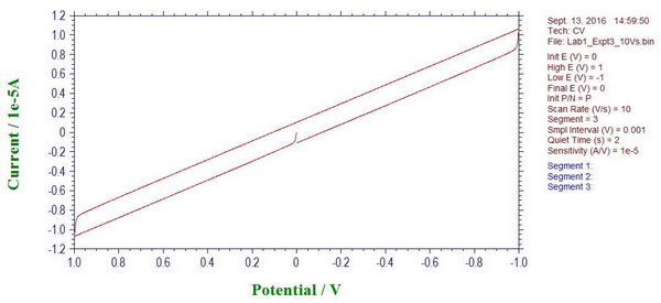
In solution, you would also see this gap, especially at very high scan rates, which results from charging the electrical double layer at the interface between electrode and electrolyte solution.
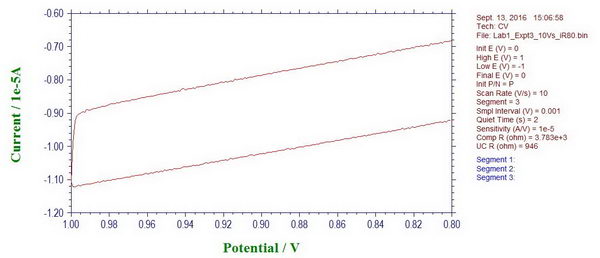
4. At this point, we can also see the effect of uncompensated solution resistance. For example, here is the moment when we change the scan direction, and it looks quite smooth, which is actually caused by the uncompensated resistance “r5” and the presence of a capacitor.
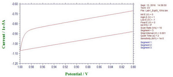
If we apply iR compensation, the potentiostat suggests resistance of ~4729 Ohm to compensate, which is almost exactly what we have there as “r5” (4.7 kOhm). When iR compensation is applied at different compensation levels (in this case, 80%), we can see how the curve becomes less smooth and ideally it should just go straight up when we change the scan polarity.
So in solution, similar effects will be observed leading to a delayed response (related to cell time constant, Ruc*Cd) with which the potential will change to the desired value (and therefore, even for fast reversible processes, you will see distortions, for example, if high resistance solution or large area electrode is used at high scan rates).
Overall, without the need to prepare any solutions, this simple equivalent circuit helps to model conditions of:
- Reaching the limit of compliance voltage
- High resistance reference electrode
- Capacitance of electrical double layer
- Uncompensated resistance
After that, we can start looking at ferrocene solutions in the next class, which is another convenient system to test all kinds of new experiments and to troubleshoot the problems.
Reading:
Zanello, P.; de Biani, F. F.; Nervi, C. “Inorganic Electrochemistry” (2011, RSC): p. 160