

Code - Fujin - Validation - Single phase flow
Laminar plane Couette flow
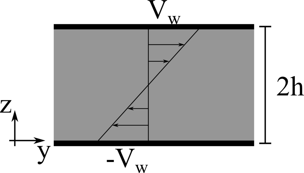
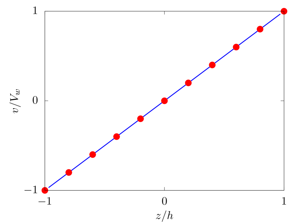
We consider the flow of a viscous fluid in a channel with moving walls, i.e., a plane Couette flow. \(x\), \(y\), and \(z\) denote the spanwise, streamwise, and wall-normal coordinates, while \(u\), \(v\), and \(w\) the corresponding components of the velocity vector field. The lower and upper impermeable moving walls are located at \(z=-h\) and \(z=h\), respectively, and move in opposite direction with constant streamwise velocity \(V_w\). The Reynolds number \(Re=\rho V_w h/ \mu\) is fixed equal to \(10\). \(32\) grid points are used to discretise the domain in the wall-normal direction.
Analytical solution: \(v \left( z \right) = -V_w \left( 1-z/h \right)\).
config.h
#define _FLOW_COUETTE_
#define _FLOW_INIT_LAMINAR_
#define _SOLVER_FFT2D_
#define _SINGLEPHASE_
parameters.f90
! Total number of grid points in X, Y and Z
integer, parameter :: nxt = 4, nyt = 4, nzt = 32
! Size of the domain in X, Y and Z
real, parameter :: lx = 0.25, ly = 0.25, lz = 2.0
! Fluid viscosity and density
real, parameter :: vis = 0.1, rho = 1.0
! Reference velocity (bulk velocity or wall velocity)
real, parameter :: refVel = 1.0
! Gravitational acceleration
real, dimension(3), parameter :: gr=(/0.0,0.0,0.0/)
input/input.in
# Simulation initial and final steps
0 100
# Simulation initial time
0.0
# Simulation initial time-step
0.0002
# Output frequency: 0D, 1D, 2D, 3D, restart data
100 100 100 1000000 1000000
# Simulation restart condition for the multiphase part
.false.
Laminar plane Poiseuille flow
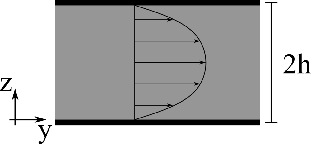
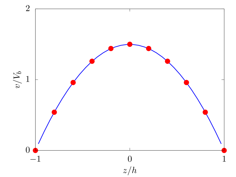
We consider the pressure-driven flow of a viscous fluid in a channel, i.e., a plane Poiseuille flow. \(x\), \(y\), and \(z\) denote the spanwise, streamwise, and wall-normal coordinates, while \(u\), \(v\), and \(w\) the corresponding components of the velocity vector field. The lower and upper impermeable walls are located at \(z=-h\) and \(z=h\), respectively, and the imposed pressure gradient maintains a constant bulk velocity \(V_b\). The Reynolds number \(Re=\rho V_b h/\mu\) is fixed equal to \(10\). \(32\) grid points are used to discretise the domain in the wall-normal direction.
Analytical solution: \(v \left( z \right) = 6 V_b \left( z/2h \right)\left[ 1- \left( z/2h \right) \right]\).
config.h
#define _FLOW_CHANNEL_
#define _FLOW_CHANNEL_CFR_
#define _FLOW_INIT_LAMINAR_
#define _SOLVER_FFT2D_
#define _SINGLEPHASE_
parameters.f90
! Total number of grid points in X, Y and Z
integer, parameter :: nxt = 4, nyt = 4, nzt = 32
! Size of the domain in X, Y and Z
real, parameter :: lx = 0.25, ly = 0.25, lz = 2.0
! Fluid viscosity and density
real, parameter :: vis = 0.1, rho = 1.0
! Reference velocity (bulk velocity or wall velocity)
real, parameter :: refVel = 1.0
! Gravitational acceleration
real, dimension(3), parameter :: gr=(/0.0,0.0,0.0/)
input/input.in
# Simulation initial and final steps
0 100
# Simulation initial time
0.0
# Simulation initial time-step
0.0002
# Output frequency: 0D, 1D, 2D, 3D, restart data
100 100 100 1000000 1000000
# Simulation restart condition for the multiphase part
.false.
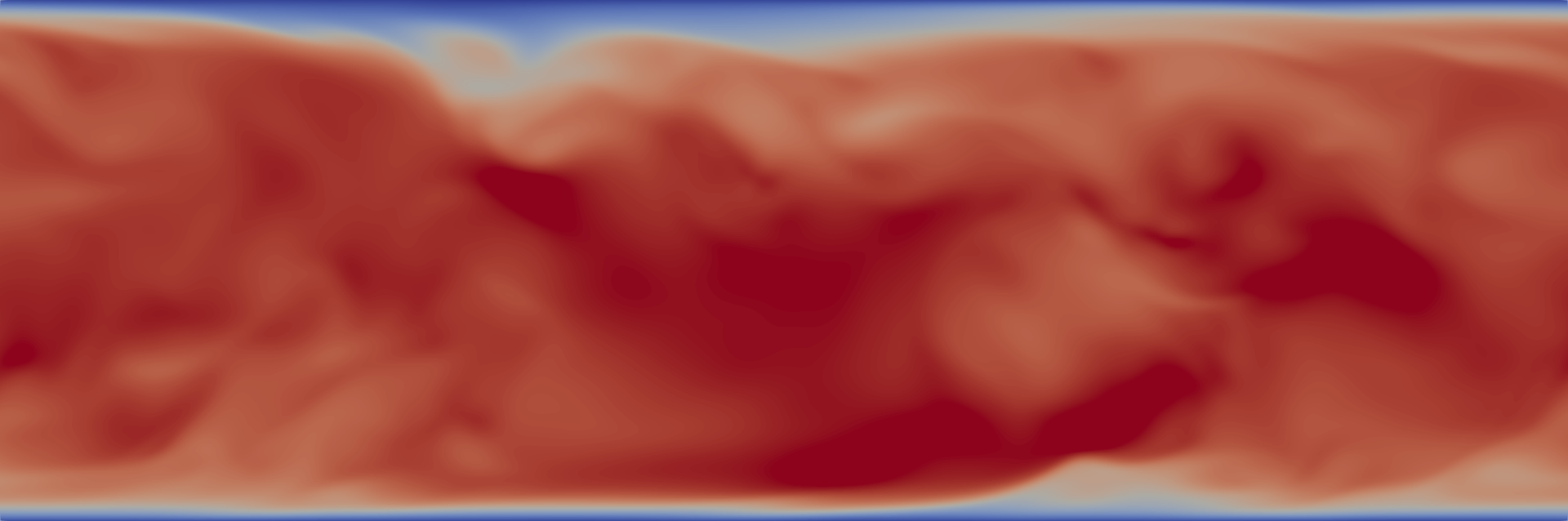
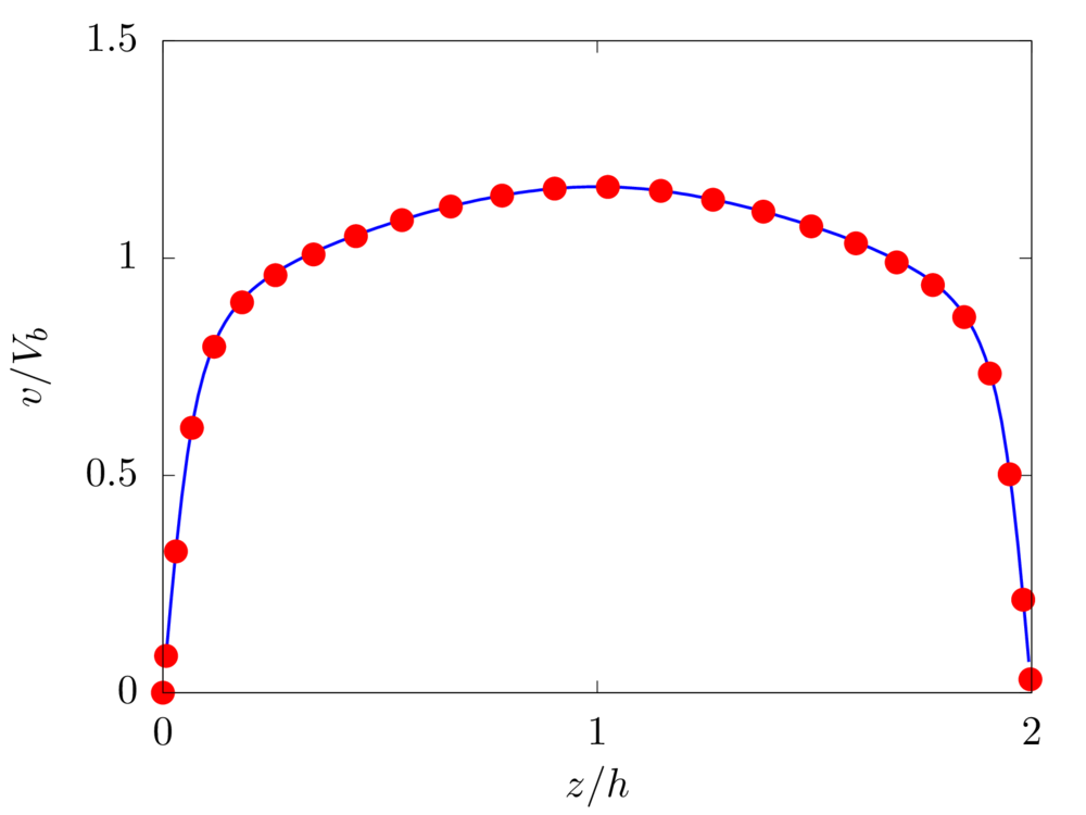
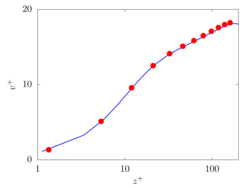
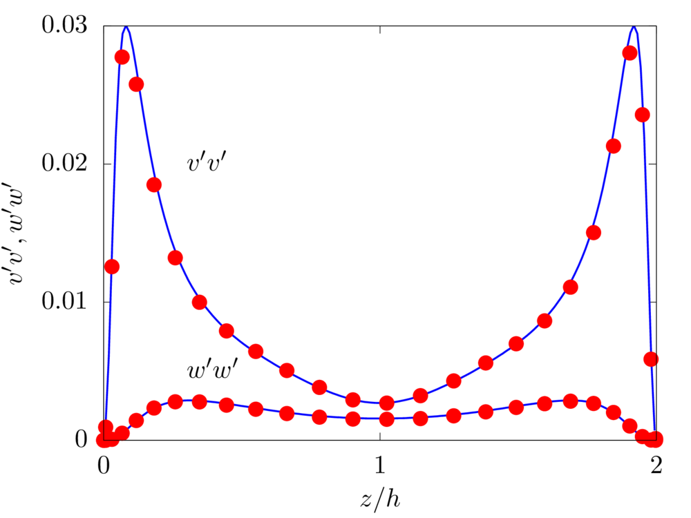
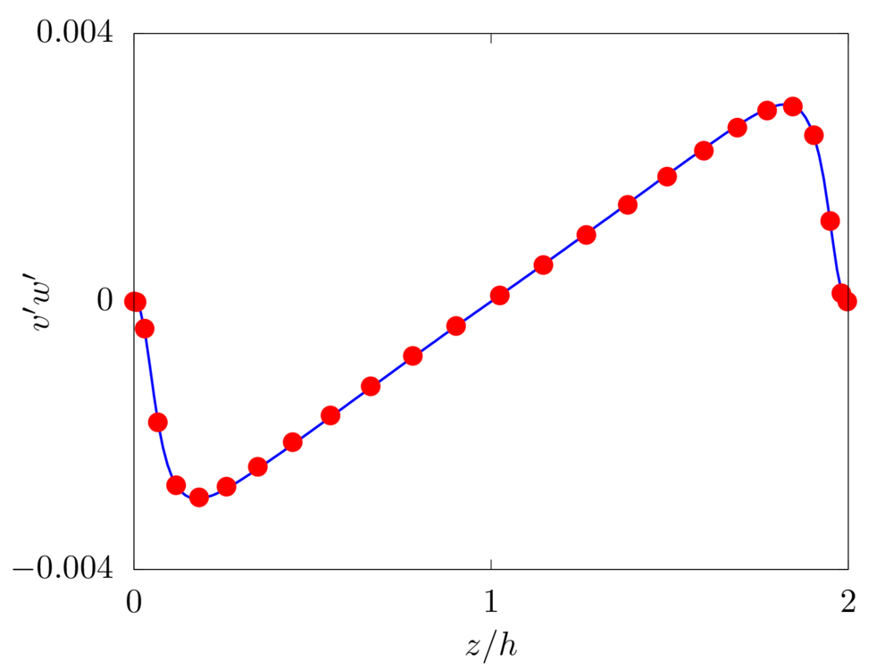
Turbulent plane channel flow
We consider the pressure-driven flow of a viscous fluid in a channel, i.e., a plane Poiseuille flow. \(x\), \(y\), and \(z\) denote the spanwise, streamwise, and wall-normal coordinates, while \(u\), \(v\), and \(w\) the corresponding components of the velocity vector field. The numerical domain has size \(3h \times 6h \times 2h\), with the lower and upper impermeable walls located at \(z=-h\) and \(z=h\), respectively. \(256 \times 512 \times 160\) grid points are used to discretise the domain. The imposed pressure gradient maintains a constant bulk velocity \(V_b\), resulting in a Reynolds number \(Re = \rho V_b h/\mu\) equal to \(2800\). The simulation is initialized with a streamwise vortex pair [1] which effectively triggers the transition to turbulence. Statistics are collected after an initial transient of \(200h/V_b\) and the results are the ensemble-average of \(900\) samples, over a period of \(1800h/V_b\).
config.h
#define _FLOW_CHANNEL_
#define _FLOW_CHANNEL_CFR_
#define _FLOW_INIT_TURBULENT_
#define _SOLVER_FFT2D_
#define _SINGLEPHASE_
parameters.f90
! Total number of grid points in X, Y and Z
integer, parameter :: nxt = 256, nyt = 512, nzt = 160
! Size of the domain in X, Y and Z
real, parameter :: lx = 3.0, ly = 6.0, lz = 2.0
! Fluid viscosity and density
real, parameter :: vis = 2.0/5600.0, rho = 1.0
! Reference velocity (bulk velocity or wall velocity)
real, parameter :: refVel = 1.0
! Gravitational acceleration
real, dimension(3), parameter :: gr=(/0.0,0.0,0.0/)
input/input.in
# Simulation initial and final steps
0 9999999
# Simulation initial time
0.0
# Simulation initial time-step
0.002
# Output frequency: 0D, 1D, 2D, 3D, restart data
100 1000 2000 1000000 10000
# Simulation restart condition for the multiphase part
.false.
ABC flow
We consider the Arnold-Beltrami-Childress (ABC) flow in a three-periodic domain of size \(2\pi L\). The velocity field is initialized as
\(u = \overline{V} \left[ \sin \left( z/L \right) + \cos \left( y/L \right) \right],\)
\(v = \overline{V} \left[ \sin \left( x/L \right) + \cos \left( z/L \right) \right],\)
\(w = \overline{V} \left[ \sin \left( y/L \right) + \cos \left( x/L \right) \right].\)
The Reynolds number \(Re = \rho \overline{V} L /\mu\) is fixed equal to \(10\) and \(32\) grid points per side are used to discretise the numerical domain.
config.h
#define _FLOW_TRIPERIODIC_
#define _FLOW_TRIPERIODIC_ABC_
#define _FLOW_INIT_LAMINAR_
#define _SOLVER_FFT3D_
#define _SINGLEPHASE_
parameters.f90
! Total number of grid points in X, Y and Z
integer, parameter :: nxt = 32, nyt = 32, nzt = 32
! Size of the domain in X, Y and Z
real, parameter :: lx = 2.0*acos(-1.), ly = 2.0*acos(-1.), lz = 2.0*acos(-1.)
! Fluid viscosity and density
real, parameter :: vis = 0.1, rho = 1.0
! Reference velocity (bulk velocity or wall velocity)
real, parameter :: refVel = 1.0
! Gravitational acceleration
real, dimension(3), parameter :: gr=(/0.0,0.0,0.0/)
input/input.in
# Simulation initial and final steps
0 100
# Simulation initial time
0.0
# Simulation initial time-step
0.0002
# Output frequency: 0D, 1D, 2D, 3D, restart data
100 100 100 1000000 1000000
# Simulation restart condition for the multiphase part
.false.
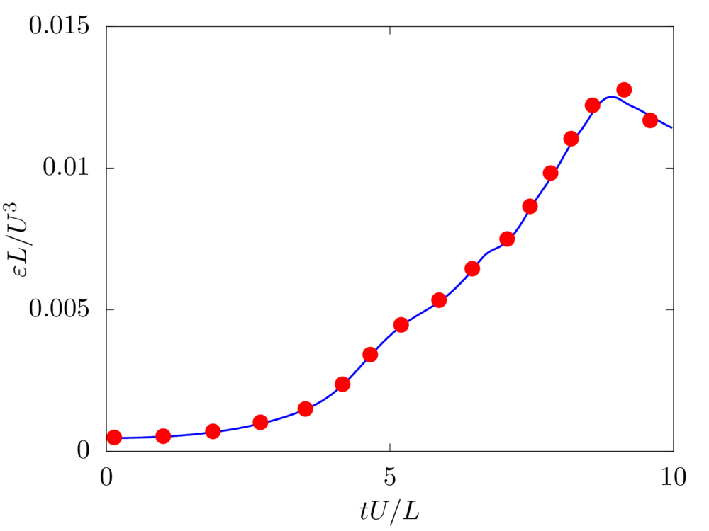
Taylor-Green Vortex
We consider the time evolution of a Taylor-Green vortex in a three-periodic domain of size \(2\pi L\). The velocity field is initialized as
\(u = U \sin \left( x/L \right) \cos \left( y/L \right) \cos \left( z/L \right),\)
\(v = -U \cos \left( x/L \right) \sin \left( y/L \right) \cos \left( z/L \right),\)
\(w=0.\)
The Reynolds number \(Re = \rho U L /\mu\) is fixed equal to \(1600\) and \(512\) grid points per side are used to discretise the numerical domain.
config.h
#define _FLOW_TRIPERIODIC_
#define _FLOW_TRIPERIODIC_TGV_
#define _FLOW_INIT_LAMINAR_
#define _SOLVER_FFT3D_
#define _SINGLEPHASE_
parameters.f90
! Total number of grid points in X, Y and Z
integer, parameter :: nxt = 512, nyt = 512, nzt = 512
! Size of the domain in X, Y and Z
real, parameter :: lx = 2.0*acos(-1.), ly = 2.0*acos(-1.), lz = 2.0*acos(-1.)
! Fluid viscosity and density
real, parameter :: vis = 1.0/1600.0, rho = 1.0
! Reference velocity (bulk velocity or wall velocity)
real, parameter :: refVel = 1.0
! Gravitational acceleration
real, dimension(3), parameter :: gr=(/0.0,0.0,0.0/)
input/input.in
# Simulation initial and final steps
0 9999999
# Simulation initial time
0.0
# Simulation initial time-step
0.0002
# Output frequency: 0D, 1D, 2D, 3D, restart data
100 1000000 1000000 1000000 10000
# Simulation restart condition for the multiphase part
.false.

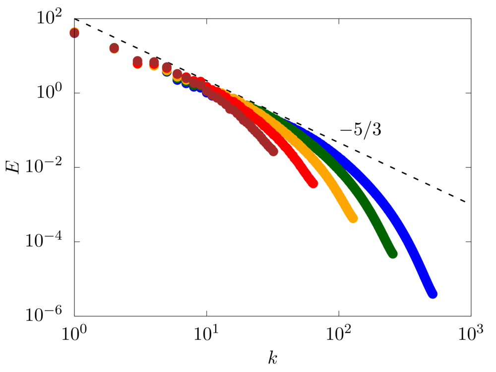
Homogeneous Isotropic Turbulence
We consider an homogeneous isotropic turbulent flow in a three-periodic domain of size \(2\pi L\). The flow is sustained by a random forcing in Fourier space [4] on wave numbers within a shell of radius \(k=2\). The Taylor microscale Reynolds number \(Re = \rho u' \lambda /\mu\) is varied from \(100\) to \(400\), and \(64\), \(128\), \(256\), \(512\) and \(1024\) grid points per side are used to discretise the numerical domain.
config.h
#define _FLOW_TRIPERIODIC_
#define _FLOW_TRIPERIODIC_ISO_
#define _FLOW_INIT_LAMINAR_
#define _SOLVER_FFT3D_
#define _SINGLEPHASE_
parameters.f90
! Total number of grid points in X, Y and Z
integer, parameter :: nxt = 1024, nyt = 1024, nzt = 1024
! Size of the domain in X, Y and Z
real, parameter :: lx = 2.0*acos(-1.), ly = 2.0*acos(-1.), lz = 2.0*acos(-1.)
! Fluid viscosity and density
real, parameter :: vis = 1.0/400.0, rho = 1.0
! Reference velocity (bulk velocity or wall velocity)
real, parameter :: refVel = 1.0
! Gravitational acceleration
real, dimension(3), parameter :: gr=(/0.0,0.0,0.0/)
input/input.in
# Simulation initial and final steps
0 9999999
# Simulation initial time
0.0
# Simulation initial time-step
0.00001
# Output frequency: 0D, 1D, 2D, 3D, restart data
100 1000000 1000000 1000000 10000
# Simulation restart condition for the multiphase part
.false.
References:
[1] D. S. Henningson and J. Kim. On turbulent spots in plane poiseuille flow. Journal of Fluid Mechanics, 228:183–205, 1991.
[2] J. Kim, P. Moin, and R. Moser. Turbulence statistics in fully developed channel flow at low Reynolds number. Journal of Fluid Mechanics, 177:133–166, 1987.
[3] W. M. Van Rees, A. Leonard, D. I. Pullin, and P. Koumoutsakos. A comparison of vortex and pseudo- spectral methods for the simulation of periodic vortical flows at high reynolds numbers. Journal of Computational Physics, 230(8):2794–2805, 2011.
[4] V. Eswaran and S. B. Pope. An examination of forcing in direct numerical simulations of turbulence. Computers & Fluids, 16(3):257–278, 1988.