

Code - Fujin - Validation - Non-Newtonian fluid
Non-Newtonian laminar plane Poiseuille flow
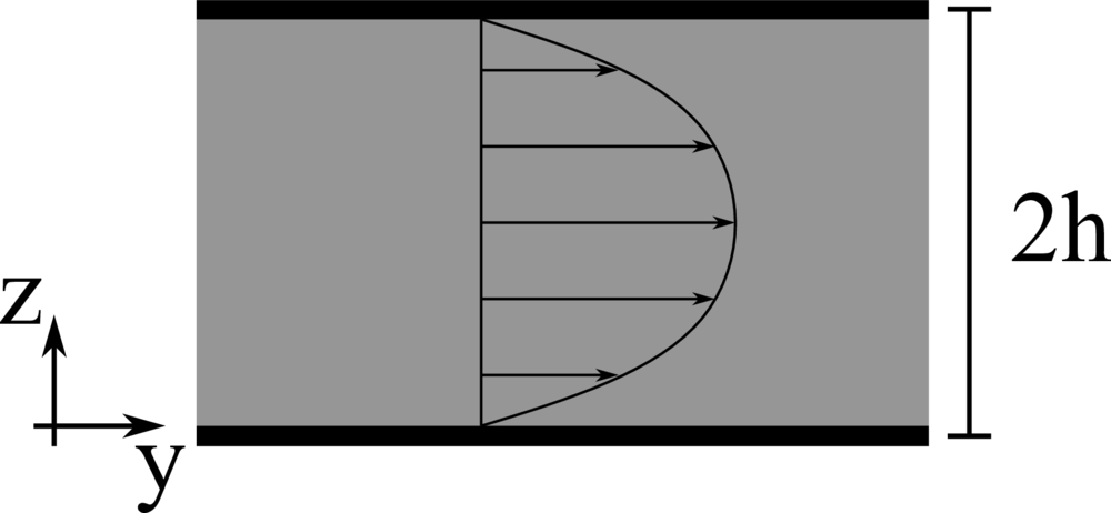
We consider the pressure-driven flow of a viscous fluid in a channel, i.e., a plane Poiseuille flow. \(x\), \(y\), and \(z\) denote the spanwise, streamwise, and wall-normal coordinates, while \(u\), \(v\), and \(w\) the corresponding components of the velocity vector field. The lower and upper impermeable walls are located at \(z=-h\) and \(z=h\), respectively, and the flow is driven by a uniform pressure gradient in the streamwise direction \(P_y\). The pressure gradient is such that with a Newtonian fluid the centerline velocity \(V_c = P_y h^2/2 \mu\) is equal to \(1\). \(32\) grid points are used to discretise the domain in the wall-normal direction. Different non-Newtonian fluids are considered.
Power-law fluid
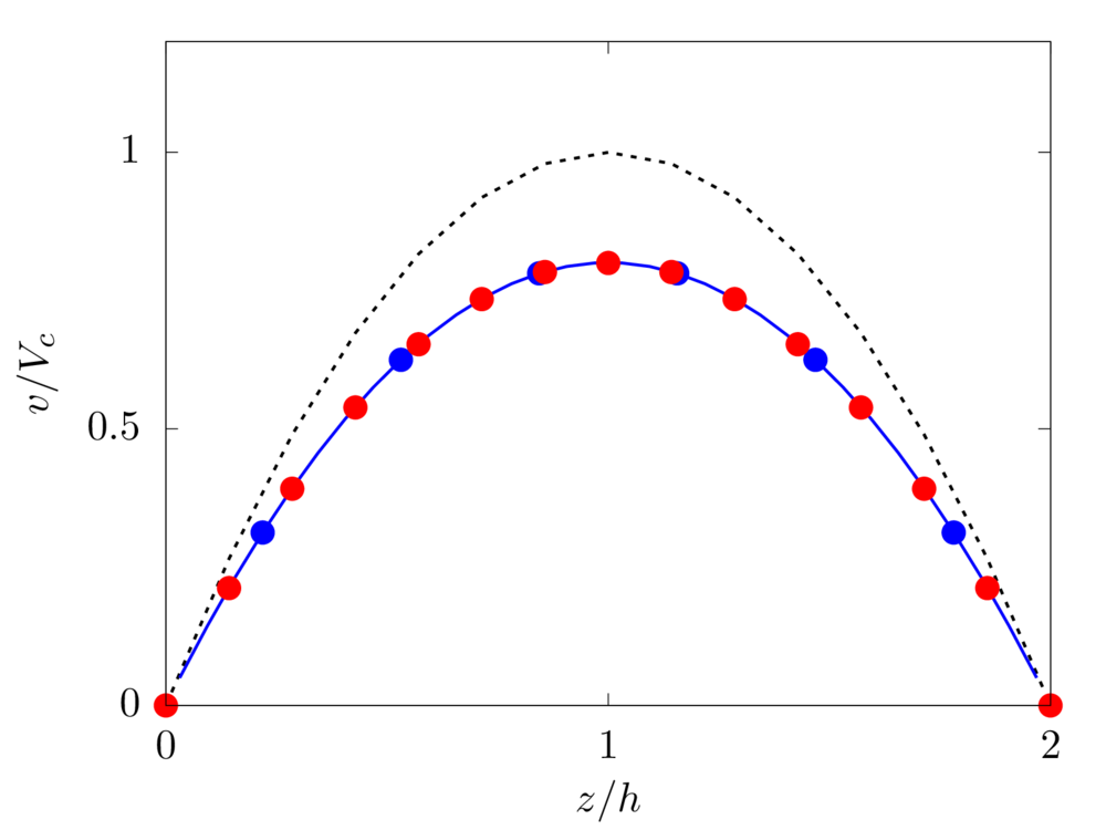
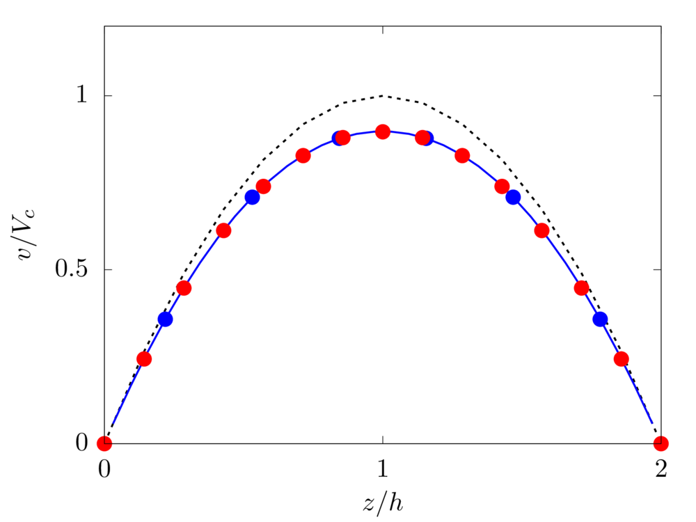
We consider shear-thinning and thickening fluids modeled as simple power-law fluids with local viscosity \(\mu_l = k \dot{\gamma}^{n-1}\), with power index \(n=0.75\) and \(1.75\), respectively, and fluid consistency index \(k\) such that \(\mu_l \left( \dot{\gamma}_0 \right)= \mu\), being \(\dot{\gamma}_0\) the mean shear rate in the channel for a Newtonian fluid, i.e. \(P_y/2 \mu h\).
Analytical solution: \(v \left( z \right) = \frac{n}{n+1} \left( \frac{P_y}{k}\right)^{\frac{1}{n}} \left[ h^\frac{n+1}{n} - \left(z-h\right)^\frac{n+1}{n} \right]\).
config.h
#define _FLOW_CHANNEL_
#define _FLOW_CHANNEL_CPG_
#define _FLOW_CHANNEL_LAMINAR_
#define _SOLVER_FFT2D_
#define _MULTIPHASE_
#define _MULTIPHASE_NNF_
#define _MULTIPHASE_VISCOSITY_VARIABLE_
#define _MULTIPHASE_DENSITY_UNIFORM_
#define _MULTIPHASE_NNF_POW_
#define _MULTIPHASE_NNF_POW_C_
param.f90
! Total number of grid points in X, Y and Z
integer, parameter :: nxt = 4, nyt = 4, nzt = 32
! Size of the domain in X, Y and Z
real, parameter :: lx = 0.25, ly = 0.25, lz = 2.0
! Fluid viscosity and density
real, parameter :: vis = 0.01, rho = 1.0
! Imposed pressure gradient
real, parameter :: gradP = 0.02
! Reference velocity (bulk velocity or wall velocity)
real, parameter :: refVel = gradP/(3.0*vis)
! Gravitational acceleration
real, dimension(3), parameter :: gr=(/0.0,0.0,0.0/)
! Output frequency
integer,parameter :: iout0d = 100000, iout1d = 100000, iout2d = 10000000, iout3d = 10000000, ioutfld = 10000000
! Power-law index
real, parameter :: nn_n = 1.75 !THICK: 1.75 - THIN: 0.75
! Fluid consistency index
real, parameter :: nn_k=vis*(3.0*refVel/lz)**(1.0-nn_n)
main.f90
! Simulation initial step
iStart = 0
! Simulation final step
iEnd = 1000000
! Choose the timestep
dt = 0.0002

Oldroyd-B fluid
We consider an Oldroyd-B fluid [1] with relaxation time \(\lambda = 10\) and polymeric viscossity \(\mu_p=\mu/4\).
Analytical solution: \(v \left( z \right) = 2 P_y h^2/ \left( \mu+\mu_p \right) \left( z/2h \right)\left[ 1- \left( z/2h \right) \right]\).
config.h
#define _FLOW_CHANNEL_
#define _FLOW_CHANNEL_CPG_
#define _FLOW_CHANNEL_LAMINAR_
#define _SOLVER_FFT2D_
#define _MULTIPHASE_
#define _MULTIPHASE_NNF_
#define _MULTIPHASE_VISCOSITY_UNIFORM_
#define _MULTIPHASE_DENSITY_UNIFORM_
#define _MULTIPHASE_NNF_OLB_
param.f90
! Total number of grid points in X, Y and Z
integer, parameter :: nxt = 4, nyt = 4, nzt = 32
! Size of the domain in X, Y and Z
real, parameter :: lx = 0.25, ly = 0.25, lz = 2.0
! Fluid viscosity and density
real, parameter :: vis = 0.01, rho = 1.0
! Imposed pressure gradient
real, parameter :: gradP = 0.02
! Reference velocity (bulk velocity or wall velocity)
real, parameter :: refVel = gradP/(3.0*vis)
! Gravitational acceleration
real, dimension(3), parameter :: gr=(/0.0,0.0,0.0/)
! Output frequency
integer,parameter :: iout0d = 100000, iout1d = 100000, iout2d = 10000000, iout3d = 10000000, ioutfld = 10000000
! Polymeric viscosity and relaxation time
real, parameter :: nnVis=vis/4.0, nnLambda=10.0
main.f90
! Simulation initial step
iStart = 0
! Simulation final step
iEnd = 2000000
! Choose the timestep
dt = 0.0002
FENE-P fluid
We consider a FENE-P fluid [2] with relaxation time \(\lambda=10\), polymeric viscosity \(\mu_p=\mu/4\) and maximum dumbbell extension \(L=6\).
Analytical solution [3]: \(u= 2 P_y h^2/\mu \left( z/2h \right)\left[ 1- \left( z/2h \right) \right] + 3/(8 C \mu) (A_+^{1/3} B_- - C_+^{1/3} D_- + A_-^{1/3} B_+ - C_-^{1/3} D_+)\),
where
\(A_\pm = Bh \pm \sqrt{B^2h^2 + A^3}\),
\(B_\pm = 3Bh \pm \sqrt{B^2h^2 + A^3}\),
\(C_\pm = B \left( z-1\right) \pm \sqrt{B^2\left( z-1\right)^2 + A^3}\),
\(D_\pm = 3 B \left( z-1\right) \pm \sqrt{B^2 \left( z-1\right)^2 + A^3}\),
with
config.h
#define _FLOW_CHANNEL_
#define _FLOW_CHANNEL_CPG_
#define _FLOW_CHANNEL_LAMINAR_
#define _SOLVER_FFT2D_
#define _MULTIPHASE_
#define _MULTIPHASE_NNF_
#define _MULTIPHASE_VISCOSITY_UNIFORM_
#define _MULTIPHASE_DENSITY_UNIFORM_
#define _MULTIPHASE_NNF_FEN_
param.f90
! Total number of grid points in X, Y and Z
integer, parameter :: nxt = 4, nyt = 4, nzt = 32
! Size of the domain in X, Y and Z
real, parameter :: lx = 0.25, ly = 0.25, lz = 2.0
! Fluid viscosity and density
real, parameter :: vis = 0.01, rho = 1.0
! Imposed pressure gradient
real, parameter :: gradP = 0.02
! Reference velocity (bulk velocity or wall velocity)
real, parameter :: refVel = gradP/(3.0*vis)
! Gravitational acceleration
real, dimension(3), parameter :: gr=(/0.0,0.0,0.0/)
! Output frequency
integer,parameter :: iout0d = 100000, iout1d = 100000, iout2d = 10000000, iout3d = 10000000, ioutfld = 10000000
! Polymeric viscosity and relaxation time
real, parameter :: nnVis=vis/4.0, nnLambda=10.0
! FENE-P dumbbell extensibility
real, parameter :: nnL2=6.0**2
main.f90
! Simulation initial step
iStart = 0
! Simulation final step
iEnd = 2000000
! Choose the timestep
dt = 0.0002
Elastoviscoplatic fluid
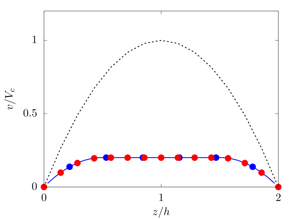
We consider an elastoviscoplastic fluid modelled with the Saramito model [4]. We fix the relaxation time \(\lambda=0.01\), polymeric viscosity \(\mu_p=\mu/4\) and yield stress \(\tau_0 = 0.01\). Due to the low value of \(\lambda\) considered, we compare the result with the purely viscoplastic solution.
Analytical solution: \(v \left( z \right) = P_y/2 \left( \mu + \mu_p \right) \left[ (z-1)^2 - h^2 \right] + \tau_0/ \left( \mu + \mu_p \right) \left[ (z-1) -h \right]\) if \(z_0 \le z-1 \lt h\) else \(v \left( z \right) = v \left( z_0+1 \right)\).
config.h
#define _FLOW_CHANNEL_
#define _FLOW_CHANNEL_CPG_
#define _FLOW_CHANNEL_LAMINAR_
#define _SOLVER_FFT2D_
#define _MULTIPHASE_
#define _MULTIPHASE_NNF_
#define _MULTIPHASE_VISCOSITY_UNIFORM_
#define _MULTIPHASE_DENSITY_UNIFORM_
#define _MULTIPHASE_NNF_EVP_
param.f90
! Total number of grid points in X, Y and Z
integer, parameter :: nxt = 4, nyt = 4, nzt = 32
! Size of the domain in X, Y and Z
real, parameter :: lx = 0.25, ly = 0.25, lz = 2.0
! Fluid viscosity and density
real, parameter :: vis = 0.01, rho = 1.0
! Imposed pressure gradient
real, parameter :: gradP = 0.02
! Reference velocity (bulk velocity or wall velocity)
real, parameter :: refVel = gradP/(3.0*vis)
! Gravitational acceleration
real, dimension(3), parameter :: gr=(/0.0,0.0,0.0/)
! Output frequency
integer,parameter :: iout0d = 100000, iout1d = 100000, iout2d = 10000000, iout3d = 10000000, ioutfld = 10000000
! Polymeric viscosity and relaxation time
real, parameter :: nnVis=vis/4.0, nnLambda=10.0/1000.0
! Yield stress (tautau0 fluid-like behaviour)
real, parameter :: nnTau0=0.01
main.f90
! Simulation initial step
iStart = 0
! Simulation final step
iEnd = 2000000
! Choose the timestep
dt = 0.0002
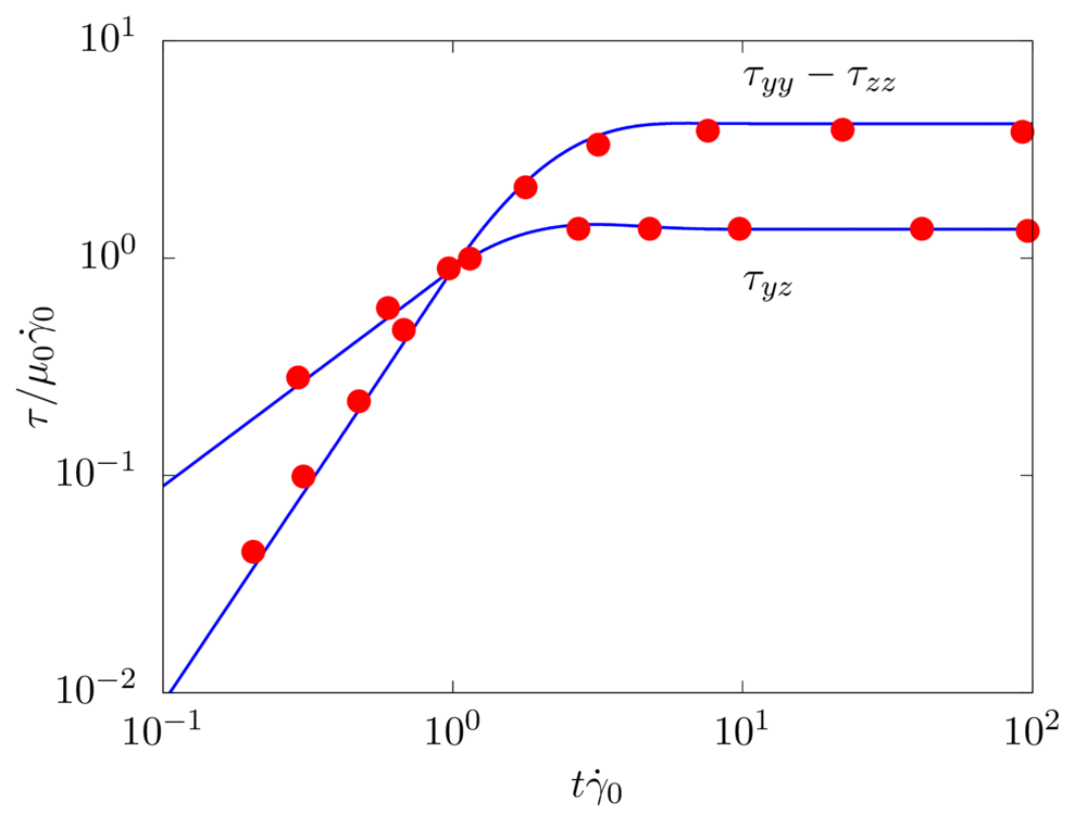
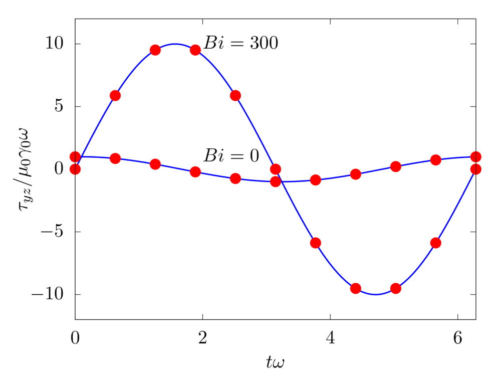
Steady and periodic shear flow with EVP fluid
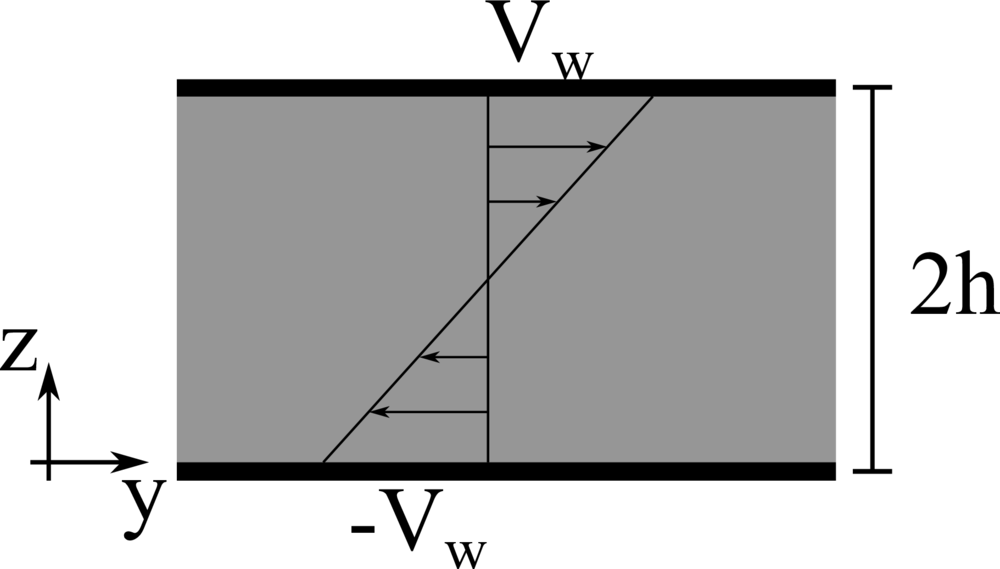
First, we consider a simple constant shear flow, with the shear rate \(\dot{\gamma}_0\): the Weissenberg number is fixed to \(Wi = \lambda \dot{\gamma}_0 = 1\), the Bingham number \(Bi = \tau_0 / \left[ \left( \mu+\mu_p \right) \dot{\gamma}_0 \right] = 1\), and the viscosity ratio \(\beta = \mu / \left( \mu + \mu_p \right) =1/9\).
Next, we consider a time-periodic uniform shear flow, i.e. \(\gamma_0 \sin \left( \omega_0 t \right)\), where \(\gamma_0\) is the strain amplitude and \(\omega_0\) the angular frequency of the oscillations. The Weissenberg number is \(Wi = \lambda \omega_0 = 0.1\) and two Bingham numbers \(Bi = \tau_0/\left[ \left( \mu + \mu_p \right) \gamma_0 \omega_0 \right]\) are considered: \(Bi = 0\) and \(300\). Note that, when \(Bi = 0\), the material behaves like a viscoelastic fluid, and when \(Bi = 300\) as an elastic solid. The viscosity ratio \(\beta = \mu / \left( \mu + \mu_p \right)\) is null in both cases, i.e. \(\mu = 0\).
config.h
#define _FLOW_CHANNEL_
#define _FLOW_FIXED_
#define _SOLVER_FFT2D_
#define _MULTIPHASE_
#define _MULTIPHASE_NNF_
#define _MULTIPHASE_VISCOSITY_UNIFORM_
#define _MULTIPHASE_DENSITY_UNIFORM_
#define _MULTIPHASE_NNF_EVP_
param.f90
! Total number of grid points in X, Y and Z
integer, parameter :: nxt = 4, nyt = 64, nzt = 64
! Size of the domain in X, Y and Z
real, parameter :: lx = 1.0, ly = 1.0, lz = 1.0
! Fluid viscosity and density
real, parameter :: vis = 0.0, rho = 1.0 !Steady: 1.0/9.0, 1.0 - Oscillating: 0.0, 1.0
! Reference velocity (bulk velocity or wall velocity)
real, parameter :: refVel = 0.5
! Gravitational acceleration
real, dimension(3), parameter :: gr=(/0.0,0.0,0.0/)
! Output frequency
integer,parameter :: iout0d = 10, iout1d = 10000000, iout2d = 10000000, iout3d = 10000000, ioutfld = 10000000
! Polymeric viscosity and relaxation time
real, parameter :: nnVis=1.0, nnLambda=0.1 !Steady: 8.0/9.0, 1.0 - Oscillating: 1.0, 0.1
! Yield stress (tautau0 fluid-like behaviour)
real, parameter :: nnTau0=300.0 !Steady: 1.0 - Oscillating: 0.0/300.0
main.f90
! Simulation initial step
iStart = 0
! Simulation final step
iEnd = 1000000
! Choose the timestep
dt = 0.001
References:
[1] J. G. Oldroyd. On the formulation of rheological equations of state. In Proceedings of the Royal Society of London A: Mathematical, Physical and Engineering Sciences, volume 200, pages 523–541. The Royal Society, 1950.
[2] A. Peterlin. Hydrodynamics of macromolecules in a velocity field with longitudinal gradient. Journal of Polymer Science: Polymer Letters, 4(4):287–291, 1966.
[3] D. O. A. Cruz, F. Pinho, and P. J. Oliveira. Analytical solutions for fully developed laminar flow of some viscoelastic liquids with a newtonian solvent contribution. Journal of Non-Newtonian Fluid Mechanics, 132(1-3):28–35, 2005.
[4] P. Saramito. A new constitutive equation for elastoviscoplastic fluid flows. Journal of Non-Newtonian Fluid Mechanics, 145(1):1–14, 2007.