1 This GUI was developed by MATLAB R2018b. We strongly suggest that you install this version before using the software. The examples of images which were converted from “tif” to “jpg” format, can be downloaded from here. The binarized images are also available here.
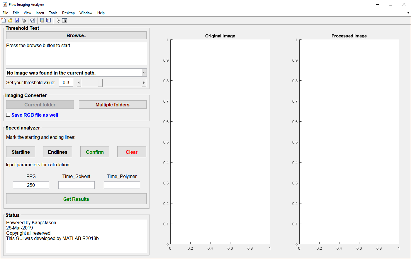
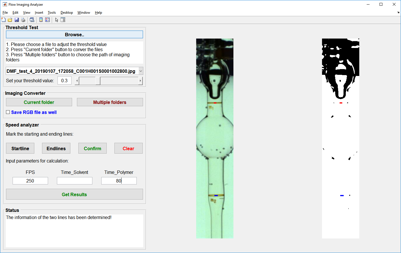
2This is an analysis based on simple binarization. The picture below shows the overview of the GUI. The download links are listed below. If you get any problems or bugs while using it, please contact me through kang-yu.chu2@oist.jp
3Before starting the analysis, we need to convert the images (the format of our original images is tiff) with a proper threshold value. We offer two ways to convert the image set. One is folder to folder, the other is multiple folder output.
3.1Folder to folder operation
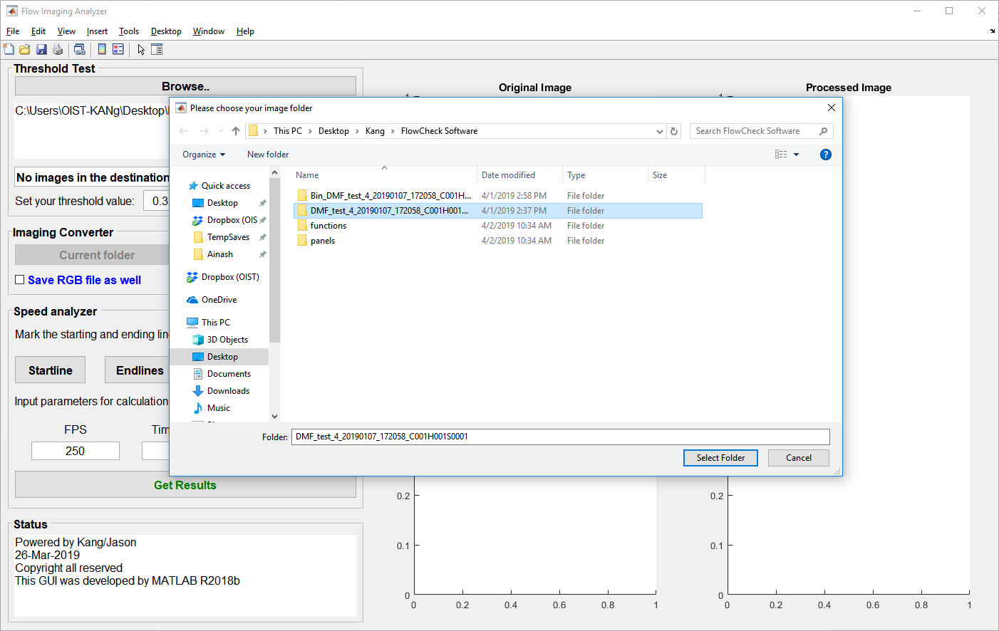
3.1.1Browse the folder of your images (we only support “tif” and “jpg”) by pressing button “Browse..”. Then, choose the folder named “DMF_test4_4…”.
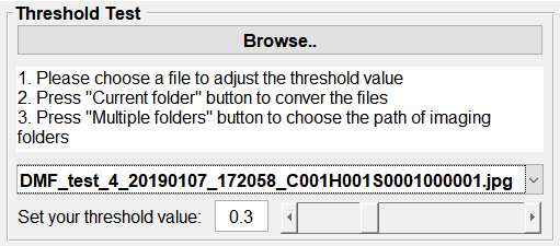
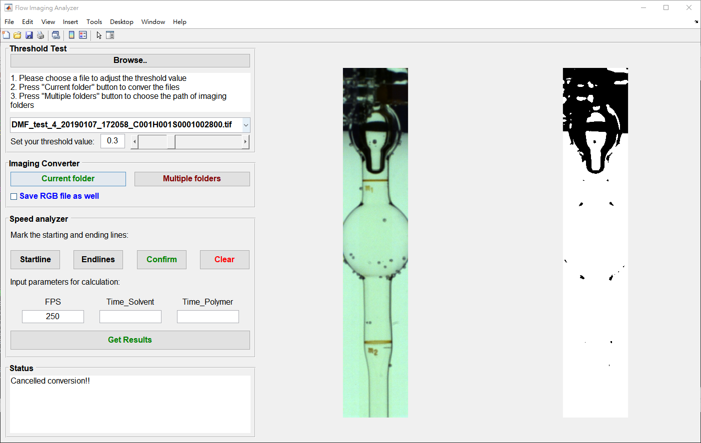
3.1.2If the folder contains files whose format is tif or jpg, it should show up in the dropdown menu like the picture bellowed. You can now select any images to start the test of the threshold value.
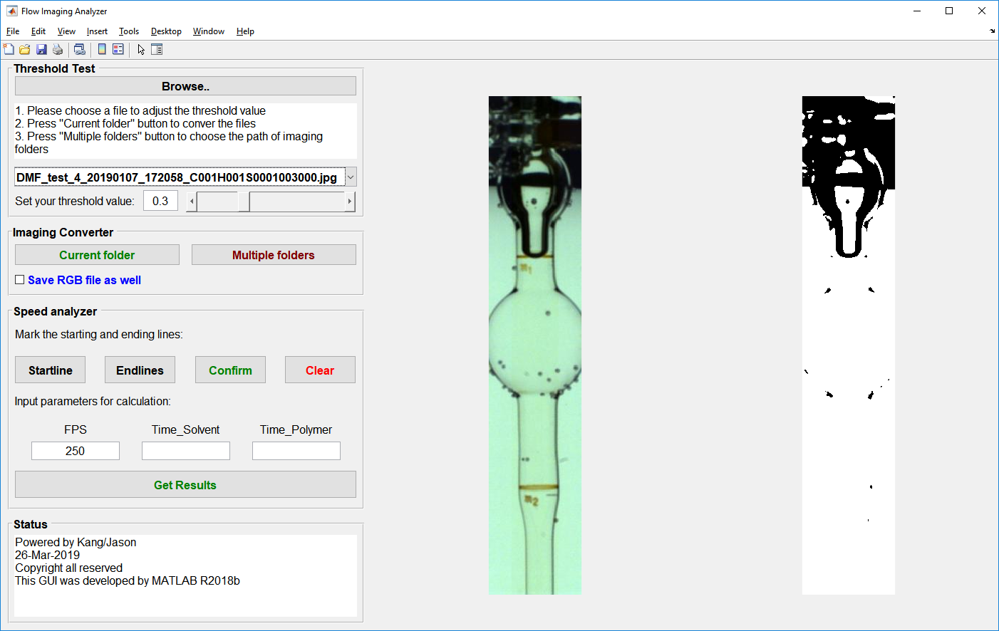
3.1.3Try to identify a proper threshold to make the passing route of fluidics cleared (without any black dot). Note that this is just the preview of your binarized images.
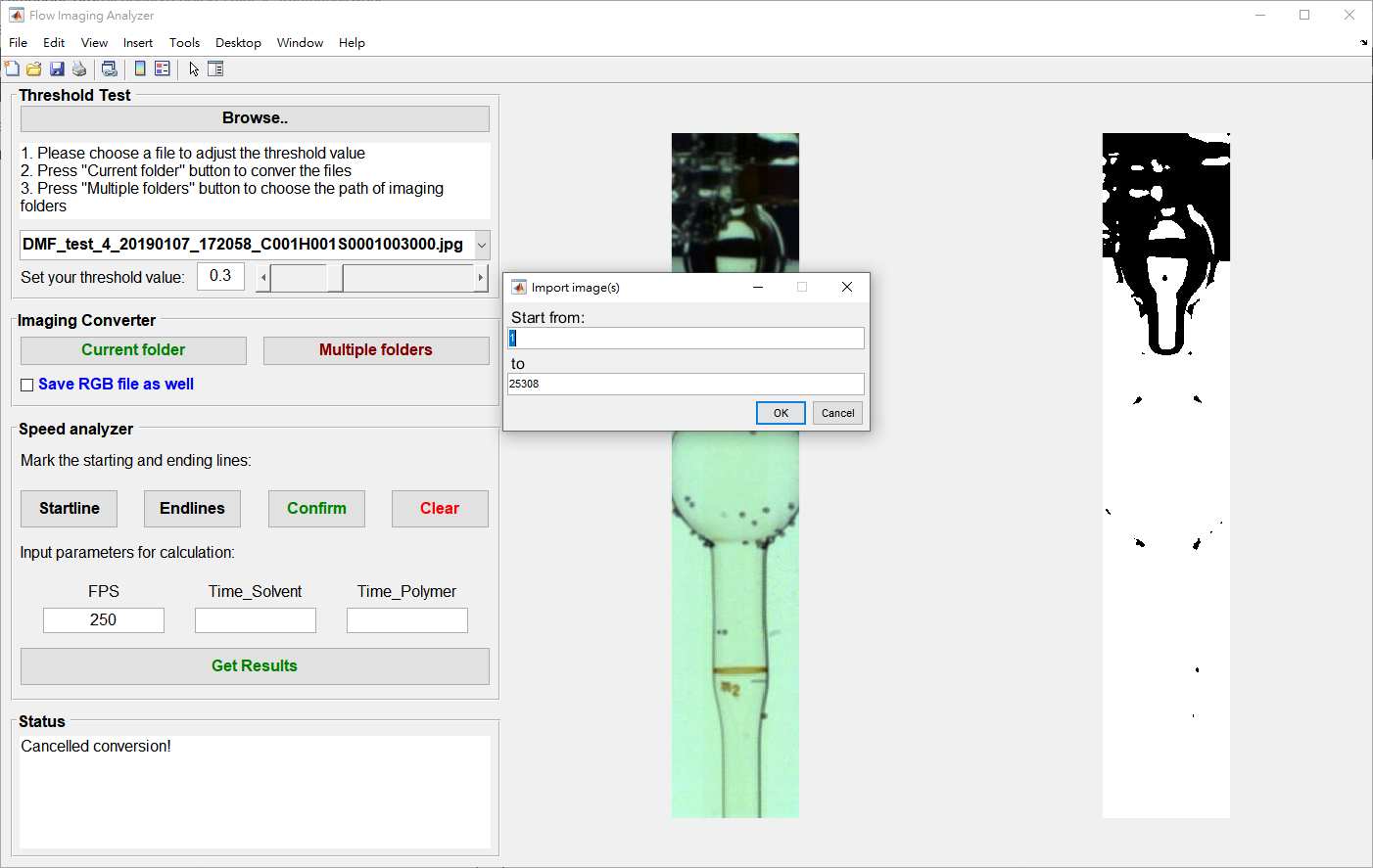
3.1.4Press “Current folder” to convert all the images in the folder. The option “Save RGB file as well” only works when the format of your images is tif. You can enter your desired interval to control, then press OK and select your output folder.
3.1.5 Wait until the status box shows “Conversion over!”.
3.2Converting multiple folders
3.2.1This function can be activated right after the program started. After setting your threshold value, you can press the “Multiple folders” to choose the path of your imaging folders.
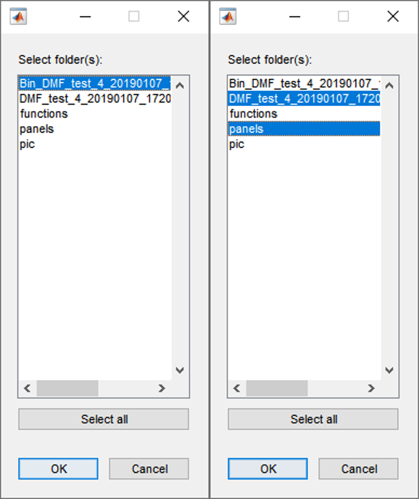
3.2.2Next, you will see a pop-up window which you can select one or multiple folders (ctrl + left click) to convert. Press ok to select the path for multiple folder output.
3.2.3Wait until the status box shows “Conversion over!”.
4Flow speed analyzer
4.1Browse the folder of the original source
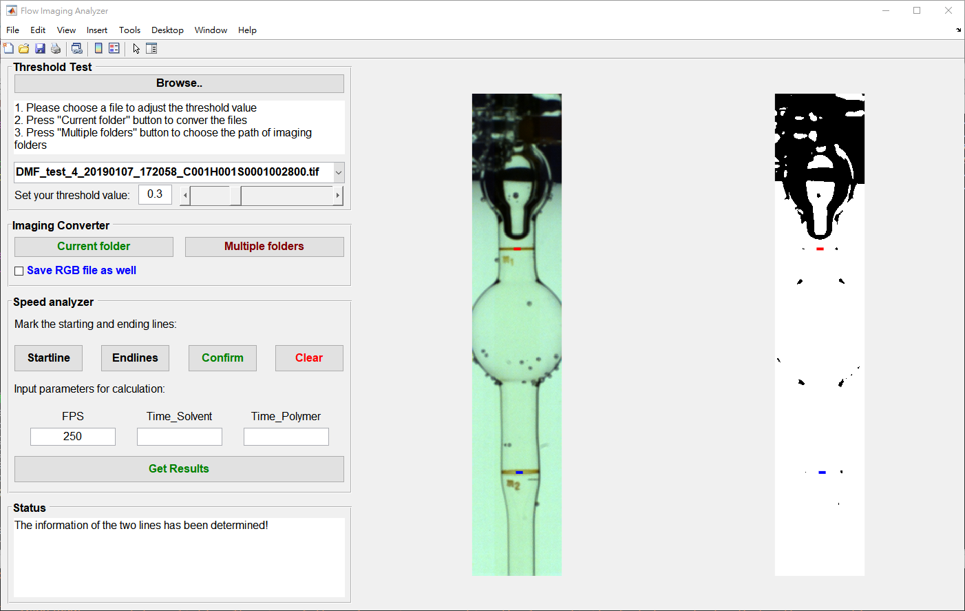
4.2Now, we will mark the start and end line for measuring the speed. Before pressing the “Startline” button, we suggest you zoom in the picture. When you move your cursor to the picture, you can see there is a toolbox on the right top side of the picture like this . Press “Startline” to select points and draw a line. The determination of end line is same as start line.
4.3Press “Confirm” button will define the detecting area. Press “Clear” to remove all the determined lines.
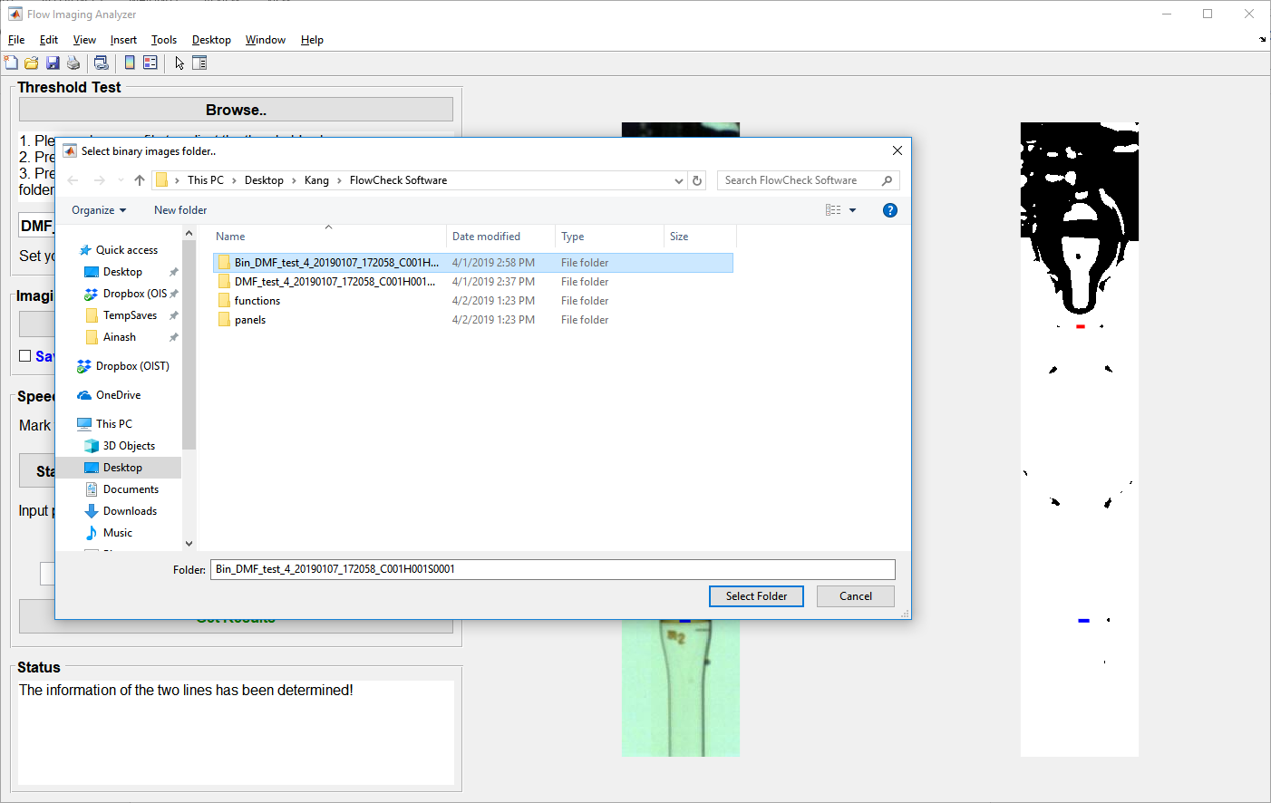
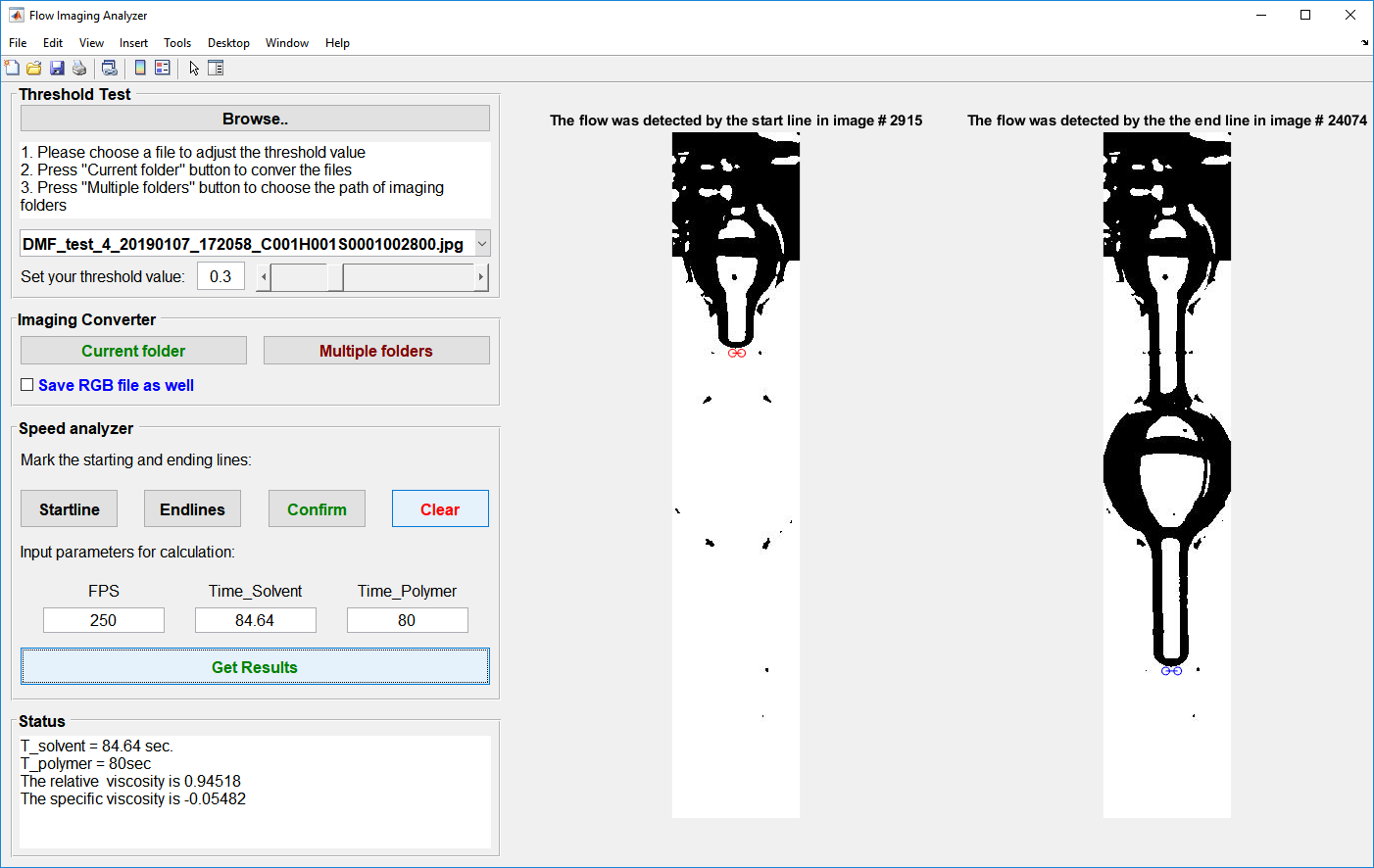
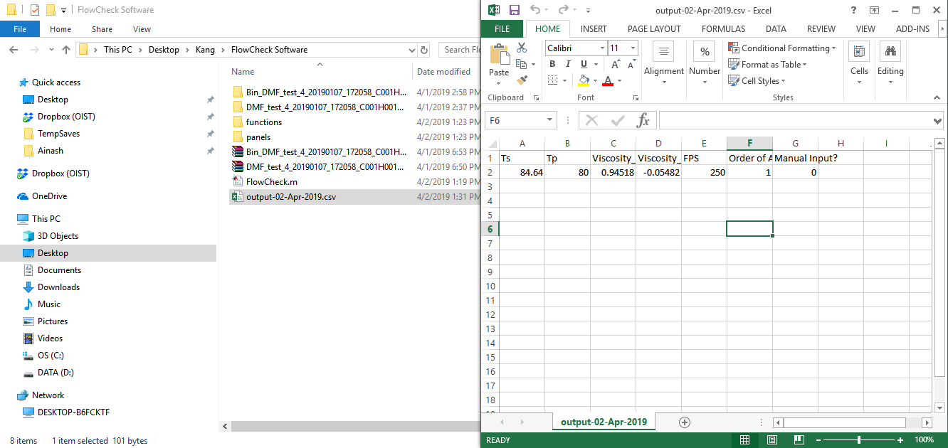
4.4You can input known values to FPS, flow time of the solvent or the polymer solution. Then, the program will automatically calculate shear viscosities and save results. Press “Get Results” and Select your converted binary images folder to start analysis.