Complex Fluids and Flows Unit (Marco Edoardo Rosti)

Code - Fujin - Validation - Volume of Fluid

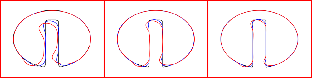
Zalesak's disk

The Zalesak’s disk [1], i.e., a slotted disk undergoing solid body rotation, is a standard benchmark to validate numerical schemes for advection problems, since the initial shape should not deform under rigid body rotation. We consider a domain of unit size with the slotted disk defined by the geometrical relation

\(\left( y -0.5 \right)^2 + \left( z - 0.75 \right)^2 \le 0.15^2 \wedge \left( \vert y - 0.5 \vert \ge 0.025 \vee z \ge 0.85 \right).\)

The velocity field is imposed equal to

\(v = 0.5 - z,\)

\(w = y - 0.5.\)

Numerical tests are carried out on three grids with \(100\), \(150\) and \(200\) grid points per side of the domain. The results are evalauted at \(t = 2 \pi\) (one revolution) and \(t = 10 \pi\) (five revolutions).

config.h

#define _FLOW_FIXED_
#define _MULTIPHASE_
#define _MULTIPHASE_VOF_
#define _MULTIPHASE_VOF_ZALESAK_
#define _MULTIPHASE_VOF_2D_
#define _MULTIPHASE_VOF_QUADRATIC_

param.f90

!Total number of grid points in X, Y and Z
integer, parameter :: nxt = 4, nyt = 100, nzt = 100
!Size of the domain in X, Y and Z
real, parameter :: lx = 4.0/100.0, ly = 1.0, lz = 1.0
!Output frequency
integer,parameter :: iout0d = 1000000, iout1d = 1000000, iout2d = 1, iout3d = 1000000, ioutfld = 1000000

main.f90

! Simulation initial step
iStart = 0
! Simulation final step
iEnd   = 400000
! Choose the timestep
dt = 0.5/(2.0*0.5/(1.0/100.0))

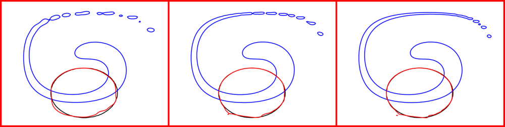
The 2D Zalesak’s disk [1]: simulation of a slotted disk undergoing solid body rotation. The black line denotes the initial solution, whereas blue and red the solutions obtained after one and five full revolutions; the results in the panels are obtained with 100, 150 and 200 grid points per domain side.

Deformed interface in a shear flow

We study a deformed interface in a shear flow in order to evaluate the capability of the method to capture a heavily deformed and stretched interface [2]. We consider a circle of radius \(0.2 \pi\), centered at \(\left[ 0.5 \pi, -0.2 \left( \pi + 1 \right) \right]\) in a box of side \(\pi\) with the prescribed velocity field

\(v = \sin \left( y \right) \cos \left( z \right),\)

\(w = -\cos \left( y \right) \sin \left( z \right).\)

First, the interface deforms due to the imposed velocity field reaching its maximum stretching at \( t = 5 \pi\) when the flow is reversed. The interface deformation starts reducing and finally, at time \(t = 10 \pi\) the interface goes back to its initial position.

config.h

#define _FLOW_FIXED_
#define _MULTIPHASE_
#define _MULTIPHASE_VOF_
#define _MULTIPHASE_VOF_DROPLETS_
#define _MULTIPHASE_VOF_2D_
#define _MULTIPHASE_VOF_QUADRATIC_

param.f90

!Total number of grid points in X, Y and Z
integer, parameter :: nxt = 4, nyt = 100, nzt = 100
!Size of the domain in X, Y and Z
real, parameter :: lx = 4.0*ACOS(-1.0)/100.0, ly = ACOS(-1.0), lz = ACOS(-1.0)
!Output frequency
integer,parameter :: iout0d = 1000000, iout1d = 1000000, iout2d = 1, iout3d = 1000000, ioutfld = 1000000

main.f90

! Simulation initial step
iStart = 0
! Simulation final step
iEnd   = 400000
! Choose the timestep
dt = 0.0025*ACOS(-1.0)

initDropletPosition.dat

1.570796326794897       0.828318530717959       0.628318530717959

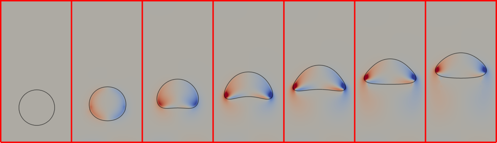
Deformed interface in a shear flow [2]: simulation of a disk undergoing forward and backward stretching. The black line denotes the initial solution at t=0, whereas blue and red the solutions obtained at t=5π and t=10π; the results in the panels are obtained with 100, 150 and 200 grid points per domain side.

Buoyancy-driven flow

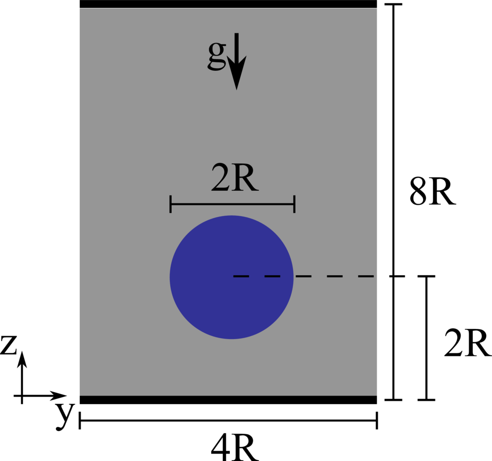
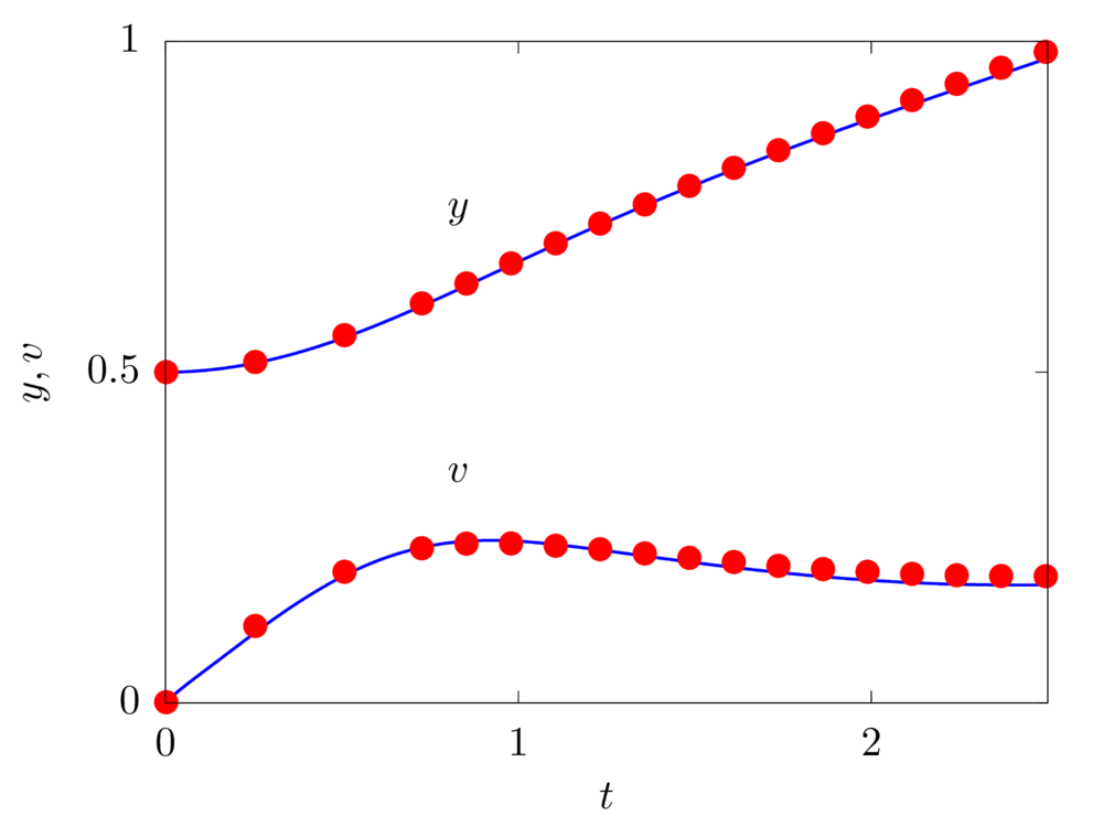
*Sketch of the computational domain and of the Cartesian coordinate system.*

We consider a 2D droplet of radius \(R\) rising in a fluid with different density and viscosity. The droplet has viscosity \(\mu_1\) and density and \(\rho_1\), while the surrounding fluid has viscosity \(\mu_2\) and density \(\rho_2\), providing a viscosity and density ratio equal to \(k_\mu = 10\) and \(k_\rho = 10\). The two fluids are separted by an interface with interfacial surface tension \(\sigma\). The domain is rectangular with size \(4 R \times 8 R\), no-slip boundary conditions are applied on the horizontal walls and free-slip boundary conditions on the sides. The droplet is initially round and placed at the centerline of the channel at a distance of \(2R\) from the bottom wall. The non-dimensional parameters governing the flow are the Reynolds number \(Re = \rho_1 U_g 2 R / \mu_1\) equal to \(35\), the Eotvos number \(Eo = \rho_1 U_g^2 2R / \sigma\) equal to \(10\), and the Capillary number \(Ca = \mu_1 U_g / \sigma\) equal to \(0.2875\), where \(U_g = \sqrt{g2R}\) being \(g\) the gravitational acceleration.

config.h

#define _FLOW_COUETTE_
#define _SOLVER_FFT2D_
#define _MULTIPHASE_
#define _MULTIPHASE_VOF_
#define _MULTIPHASE_VOF_DROPLETS_
#define _MULTIPHASE_VISCOSITY_VARIABLE_
#define _MULTIPHASE_DENSITY_VARIABLE_
#define _MULTIPHASE_VOF_2D_
#define _MULTIPHASE_VOF_QUADRATIC_

param.f90

!Total number of grid points in X, Y and Z
integer, parameter :: nxt = 4, nyt = 128, nzt = 256
!Size of the domain in X, Y and Z
real, parameter :: lx = 4.0*1.0/128.0, ly = 1.0, lz = 2.0
!Fluid viscosity and density
real, parameter :: vis = 10.0, rho = 1000.0
!Reference velocity (bulk velocity or wall velocity)
real, parameter :: refVel = 0.0
!Gravitational acceleration
real, dimension(3), parameter :: gr=(/0.0,0.0,-0.98/)
!Output frequency
integer,parameter :: iout0d = 100, iout1d = 10000, iout2d = 10000, iout3d = 10000, ioutfld = 10000
!Number of droplets
integer, parameter :: vofN = 1
!Interfacial surface tension
real, parameter :: vofSigma = 24.5
!Viscosity of the disphersed phase (phi=1)
real, parameter :: vofVis1 = 1.0
!Viscosity of the carrier phase (phi=0)
real, parameter :: vofVis2 = vis
!Density of the disphersed phase (phi=1)
real, parameter :: vofRho1 = 100.0
!Density of the carrier phase (phi=0)
real, parameter :: vofRho2 = rho

main.f90

! Simulation initial step
iStart = 0
! Simulation final step
iEnd = 9999999
! Choose the timestep
dt = 0.00001

initDropletPosition.dat

0.5 0.5 0.25

*Time evolution of the droplet shape (black line) and vorticity (color contour).*

*Center of mass position and rising speed of a 2D droplet in a Newtonian fluid. The line denotes the numerical results and the symbols those from Ref. [3].*

Droplet deformation in a shear flow

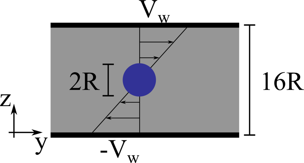
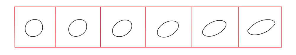
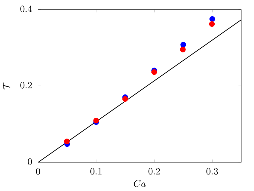
We consider a 3D spherical drop of radius \(R\) located at the center of a computational domain of size \(8R \times 16R \times 16R\), discretised with a resolution of \(20\) grid points per drop diameter. The top and bottom walls move with opposite velocity \(\pm V_w\), providing a shear rate \(\dot{\gamma} = 2 V_w/16R\), while periodic boundary conditions are imposed in the remaining directions. The same density and viscosity are specified for the spherical drop and the surrounding fluid, the Reynolds number \(Re = \rho \dot{\gamma} R^2/\mu\) is fixed to \(0.1\), and six capillary numbers are studied: \(0.05\), \(0.10\), \(0.15\), \(0.20\), \(0.25\) and \(0.30\).

config.h

#define _FLOW_COUETTE_
#define _SOLVER_FFT2D_
#define _MULTIPHASE_
#define _MULTIPHASE_VOF_
#define _MULTIPHASE_VOF_DROPLETS_
#define _MULTIPHASE_VISCOSITY_UNIFORM_
#define _MULTIPHASE_DENSITY_UNIFORM_
#define _MULTIPHASE_VOF_3D_
#define _MULTIPHASE_VOF_QUADRATIC_

param.f90

!Total number of grid points in X, Y and Z
integer, parameter :: nxt = 80, nyt = 160, nzt = 160
!Size of the domain in X, Y and Z
real, parameter :: lx = 4.0, ly = 8.0, lz = 8.0
!Fluid viscosity and density
real, parameter :: vis = 0.5**2/0.1, rho = 1.0
!Reference velocity (bulk velocity or wall velocity)
real, parameter :: refVel = 4.0
!Gravitational acceleration
real, dimension(3), parameter :: gr=(/0.0,0.0,-0.0/)
!Output frequency
integer,parameter :: iout0d = 100, iout1d = 100000, iout2d = 20000, iout3d = 100000, ioutfld = 100000
!Number of droplets
integer, parameter :: vofN = 1
!Interfacial surface tension
real, parameter :: vofSigma = vis*0.5/0.05

main.f90

! Simulation initial step
iStart = 0
! Simulation final step
iEnd = 9999999
! Choose the timestep
dt = 0.0001/2.0

initDropletPosition.dat

2.0 4.0 4.0 0.5

*The deformed interface for increasing capillary numbers.*

Taylor deformation parameter versus the capillary number. The blue symbols are the present numerical results, the red ones those by Ref. [4] and the solid line the theoretical analysis by Taylor Ref [5] on the assumptions of small deformation and Stokes flow.

References:

[1] S. T. Zalesak. Fully multidimensional flux-corrected transport. Journal of Computational Physics, 31:335–362, 1979.

[2] M. Rudman. Volume-tracking methods for interfacial flow calculations. International Journal for Nu- merical Methods in Fluids, 24(7):671–691, 1997.

[3] S. R. Hysing, S. Turek, D. Kuzmin, N. Parolini, E. Burman, S. Ganesan, and L. Tobiska. Quantitative benchmark computations of two-dimensional bubble dynamics. International Journal for Numerical Methods in Fluids, 60(11):1259-1288, 2009.

[4] S. Ii, K. Sugiyama, S. Takeuchi, S. Takagi, Y. Matsumoto, and F. Xiao. An interface capturing method with a continuous function: the THINC method with multi-dimensional reconstruction. Journal of Computational Physics, 231(5):2328–2358, 2012.

[5] G. I. Taylor. The formation of emulsions in definable fields of flow. Proceedings of the Royal Society of London A: Mathematical, Physical and Engineering Sciences, 146(858):501–523, 1934.