FY2015 Annual Report

Collective Interactions Unit
Assistant Professor Mahesh Bandi

 

Abstract

We are an experimental group with primary interests in nonlinear and non-equilibrium physics, both applied and fundamental. Our work often intersects with soft matter physics, applied mathematics, mechanics, and their application to biologically inspired problems. Our current focus is trained towards problems in interfacial fluid dynamics, granular solids, biomechanics of the human foot and fluctuations in renewable energy sources.

1. Staff

• Mr. Sahil Acharya, Rotation Student
• Dr. V. Sathish Akella, Postdoctoral Scholar
• Dr. Saikat Basu, Postdoctoral Scholar
• Mr. Kenneth J. Meacham III, Technical Staff
• Mr. Khoi D. Nguyen, Technical Staff
• Dr. Florine Paraz, Postdoctoral Scholar
• Dr. Harsha M. Paroor, Postdoctoral Scholar
• Ms. Christina Ripken, Rotation Student
• Ms. Ayano Sakiyama, Group Administrator
• Dr. Dhiraj K. Singh, Postdoctoral Scholar
• Mahesh M. Bandi, Assistant Professor

2. Collaborations

2.1 Foot in motion - materials, mechanics & control (funded by HFSP)

• Description: Theoretical, numerical and experimental studies in evolution of stiffness in the human foot.
• Type of collaboration: Joint research
• Researchers:
  • Professor Madhusudhan Venkadesan, Yale University, USA.
  • Mr. Nihav Dhavale, National Centre for Biological Sciences, India.
  • Ms. Neelima Sharma, Yale University, USA.
  • Professor Shreyas Mandre, Brown University, USA.
  • Ms. Maria Fernanda Lugo-Bolanos, Brown University, USA.
  • Professor Mahesh M. Bandi, OIST Graduate University, Japan.
  • Dr. Dhiraj K. Singha, OIST Graduate University, Japan.
  • Mr. Khoi D. Nguyen, Technical Staff, OIST Graduate University, Japan.

2.2 Compaction in two-dimensional granular materials

• Description: Compaction, disorder induced metastability, and convection in granular media..
• Type of collaboration: Joint research
• Researchers:
  • Professor Hiroaki Katsuragi, School of Environmental Sciences, Nagoya University.
  • Mr. Naoki Iikawa, School of Environmental Sciences, Nagoya University.
  • Professor Mahesh M. Bandi, OIST Graduate University, Japan.

3. Activities and Findings

3.1 Grid-scale fluctuations and forecast error in wind power

Golan Bel, Dept. of Solar Energy & Desert Research, Ben Gurion University of the Negev, Israel.

Colm P. Connaughton, Centre for Complexity Science, University of Warwick, United Kingdom

Märt Toots, Collective Interactions Unit, OIST Graduate University, Japan

Mahesh M. Bandi, Collective Interactions Units, OIST Graduate University

Renewable power generation, unlike conventional power, exhibits variability owing to natural fluctuations in the energy source, with fluctuation time scales depending on the source type. Whereas biomass and hydroelectric sources vary over long time periods, wind and solar photovoltaics exhibit short time scale variability. Wind power, in particular, shares the spectral features of the turbulent wind from which it derives energy at the scales of an individual turbine and a wind farm. This spectral correspondence implies that correlations of atmospheric turbulence are reflected in the temporal correlations of fluctuations in the generated wind power. One normally assumes that geographically distant wind farms are independent and that temporal correlations in the fluctuating wind power for each farm do not translate into long-range spatial correlations. The total power entering the grid from a large number of distant farms is expected to be much smoother and to exhibit much weaker high frequency fluctuations than the power entering from a single wind farm or a single turbine. This assumption forms the basis for proposals to interconnect local wind farms for the purpose of mitigating wind power fluctuations. Whereas fluctuations do smooth out as an increasing number of wind farms contribute to the aggregate power, it has been shown that the fluctuations are still larger than expected.

Using data from the Irish grid operator EIRGRID as a representative example, we studied the temporal correlations in the aggregate wind power entering the Irish grid. The Irish grid is fed by 224 wind farms spread across the Republic of Ireland, a much larger number of farms than the number in the aggregate power previously considered in Texas. We found that the aggregate wind power entering the Irish grid exhibits temporally correlated fluctuations with a self-similar structure.  The persistence of correlations, despite an order of magnitude increase in the number of wind farms (and their spatial distribution), strongly points to the presence of long-range spatial correlations in the atmospheric turbulence, which couples geographically distributed wind farms, thereby rendering them non-independent. These results accord with prior studies establishing the presence of long-range correlations within the mesoscale (~1-1000$ km) of atmospheric turbulence. For long time scales, these fluctuations in atmospheric flows were shown to exhibit a multi-fractal structure.

Variability adds a cost to renewable power that is absent in conventional power generation. Since an electrical grid has no storage capacity, the production and consumer demand must be balanced in real time at every instant. The grid operator purchases energy units from the producer in an energy market, from a few days to a few milliseconds in advance of delivery. With conventional energy, the grid operator must estimate in advance the consumer demand (scheduling), the estimation of which may not be trivial, and additional energy units required on standby (operating reserves). In the case of renewable energy, the operator must additionally account for both variability (fluctuations) and forecast uncertainty (error) at the production end, calling for uncertainty management in scheduling.  Furthermore, large ramps in power fluctuations, in the case of renewable energy, present the possibility of grid destabilization and blackout, a constant source of concern for grid operators. This risk further increases the cost of the operating reserves needed on standby to prevent grid failure. Naturally, forecast models constitute essential tools in estimating the magnitude of fluctuations beforehand and in planning for the optimal operating reserves required on call. Yet, no standards for forecast accuracy currently exist.

The performance of a model is often quantified by the mean and variance of the error (deviation of the prediction from the measured value). Extant works on wind power forecast error, ranging from the turbine to the grid scale, have focused on modeling the forecast error distribution.  Since a probability distribution is time-independent, it contains no information on temporal error variations. Several studies have considered the dependence of the mean and variance of the error on the duration for which the power is predicted (ranging from minutes to hours). Other works have considered the different distributions of errors for mean power over different durations. However, none of these studies account for the fluctuation correlations of the atmospheric turbulence transferred to the generated power in the analysis of forecast error or for the temporal correlations in the fluctuations and errors themselves. In this work, we suggest that the performance of wind power forecast models (as well as the performance of any model for non-stationary processes) should also account for the quality of the prediction against temporal correlations.

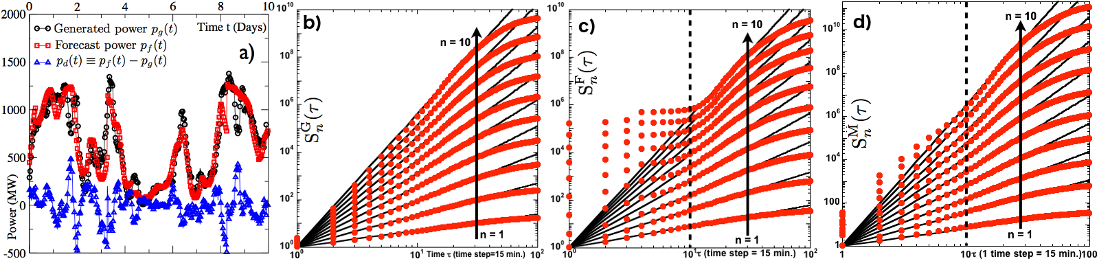
Figure 1: a) A 10 day time record of total wind power generated across Ireland, forecast, and their instantaneous difference. Structure functions quantifying the fluctuations in (b) generated wind power across Ireland, (c) forecast power, and (c) modified forecast with our model.

To analyze temporal correlations in grid-scale fluctuations for wind power, we draw upon the Statistical Theory of Hydrodynamic Turbulence to quantify two types of forecast error. The first is a timescale error (e_τ)that quantifies the timescales over which the forecast models fail to predict high frequency power fluctuations. This timescale error sets a bound on the numerical resolution of forecast models and would already be known to producers who own the farms and run the forecast models. However, model details are usually not available to grid operators who manage the supply side uncertainty. The second type of error we quantify is a scaling error (e_ζ) that establishes a difference in the self-similar scaling of fluctuations as observed for actual generated power vis à vis the power that was forecast to be generated. This error could be potentially useful to model developers, and if such an error results from large-scale correlations in atmospheric turbulence, incorporating these correlations into models is not subject to limitations arising from numerical resolution. Having established the errors, we employ a simple memory kernel upon the forecast time series and show that the errors are easily reduced with a minimal computational cost.

Two raw time series are provided by EIRGRID: the wind power generated nationwide across all Ireland entering the grid p_g(t), and the power forecast by EIRGRID's models p_f(t) for the same period. The forecast is provided for 24 hours at a time (implying different lead times for different times in the forecast series) and is based on a multi-scheme ensemble of regional weather forecast models. The time series sampled at 15-minute intervals span a five-year period (2009-2014). As we discuss in the following, we observed no change in the forecast accuracy during this five-year period.  Given that most spot markets do not trade at time scales shorter than 15 minutes, our analysis finds potential applicability in these markets, as well as in managing uncertainty over a future horizon of several hours up to a day to improve forecast models.

Raw time series for the generated power p_g(t), forecast power p_f(t), and their instantaneous difference p_d(t) = p_f(t) - p_g(t), which we define as the instantaneous forecast error, are shown in figure 1a for a 10-day period, permitting a few immediate qualitative observations. Firstly, p_g(t) exhibits correlated fluctuations. Secondly, p_f(t), while closely following p_g(t), misses the high frequency (relative to the sampling rate of the time series) components. Data analysis performed on these time series (results are shown in figure 2) yielded the quantitative estimates for timescale and scaling errors discussed above.

 

 

3.2 Variability of the wind turbine power curve

Professor Mahesh M. Bandi, Collective Interactions Unit, OIST Graduate University, Japan

Professor Jay Apt, Tepper School of Business and Depart of Engineering and Public Policy, Carnegie Mellon University, USA.

The wind turbine power curve relates the speed of wind blowing past a turbine to the power generated by the turbine. Wind plant operators forecast the power they expect to generate by feeding wind speed forecasts from numerical weather models to these power curves. The power curves are supplied to operators by turbine manufacturers who calibrate them under standards specified by the International Electrotechnical Commission (IEC64100-12-1). The IEC standard considers the average behaviour between the mean wind speed and mean power output, hence does not locally hold in time for instantaneous measurements. Indeed, instantaneous values of wind speed v(t) and wind power P(t) exhibit significant scatter about the mean profile (figure 1). Several studies have focused on the factors contributing to this variability, including turbulent fluctuations, wind shear, directional shear, directional fluctuations etc. with the aim to accurately model the "mean'' profile of the wind turbine power curve.

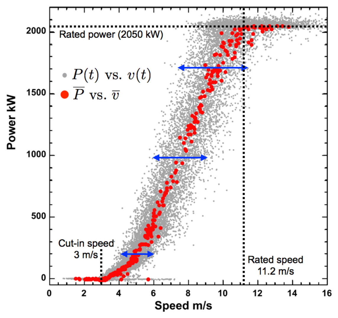
Figure 1: Instantaneous power P(t) versus instantaneous wind speed v(t) in solid grey circles and time-averaged power versus time-averaged wind speed in solid red circles for 2.05 MW MM92 turbine in Howard, NY. Considerable scatter in P(t) versus v(t) occurs about the time-averaged power curve. The scatter increases with mean speed as qualitatively shown with blue arrows at v = 5, 7 and 9 m/s.

 

This work presents a minimal parameter description of wind speed variability and wind power variability in terms of the mean wind speed. Our objective here is to remain faithful to the IEC standard (IEC64100-12-1) that prescribes the power curve with mean wind speed as its only parameter. We present empirical evidence that the standard deviation in wind speed systematically varies with mean wind speed. At least in some instances, this monotonic variation follows algebraic scaling of the form, which we attribute to residual signal correlations that remain post averaging, then affords a description of mean wind power and its standard deviation in terms of alone.

 

Our analysis of wind data obtained from three different planetary locations reveals that in instances when this scaling form is satisfied, the power-law exponent varies with geographic location, and hence must reflect local environmental factors not captured by manufacturer supplied calibration power curves. Consequently, when these calibration power curves are applied to forecast wind power, wind speed variability transforms into power forecast uncertainty. Since the variability always increases in tandem with mean speed, the resulting forecast error is multiplicative, so it substantially increases uncertainty in wind power forecasts. We conclude with a proposal that wind plant operators should recalibrate turbine power curves at the plant location to properly account for variability arising from local environmental factors. This will help reduce the uncertainty of wind power forecasts.

 

Whereas the IEC standard considers only mean quantities, as we show below, both mean power output and its standard deviation strongly depend upon wind speed variability, in addition to mean wind speed. Strong local environmental dependence of wind speed fluctuations naturally affects both the mean profile of the power curve and its variability. When not properly accounted for, this increases forecast uncertainty, which in turn adds costs to renewable energy production. Understanding the source of variability and utilising it appropriately therefore brings tangible benefits to the global renewable energy community.

3.2 (Hydro)Dynamics of self-propelled camphor boats at air-water interfaces.

Dr. V. Sathish Akella, Collective Interactions Unit, OIST Graduate University, Japan

Dr. Dhiraj K. Singh, Collective Interactions Unit, OIST Graduate University, Japan

Dr. Ravi S. Singh, School of Engineering, Brown University, USA.

Professor Shreyas Mandre, School of Engineering, Brown University, USA.

Professor Mahesh Bandi, School of Engineering, Brown University, USA.

Studies on the self-motion of camphor at air-water interfaces have a distinguished history in the annals of science. Between first observations reported in 1686 to eventually explaining camphor self-motion as resulting from surface tension gradients in 1869, the problem attracted the attention of some of the finest scientific minds including Alessandro Volta, Giovanni Battista Venturi, Jean-Baptiste Biot and Lord Rayeligh amongst others. Despite its rich history, the camphor boat system continues to remain relevant into modern times, be it in statistical mechanics within the context of active matter, hydrodynamic context of viscous marangoni propulsion, biological context of chemomechanical transduction, autonomous motion and self-assembly, and reconfigurable actuators in soft matter physics among many others.

In this work, we conducted an experimental study of the self-motion of agarose gel tablets loaded with camphoric acid (CA) at the air-water interface, henceforth referred to as c-boats. We identified three distinct modes of motion, namely a harmonic mode where the c-boat speed undergoes temporal sinusoidal oscillations, a steady mode of constant c-boat motion, and a relaxation oscillation mode where the c-boat remains at rest between sudden jumps in speed and position at regular time intervals. Whereas all three modes have been separately reported in the published record in a variety of systems, we show these seemingly different self-propulsive modes arise from a common description. Through metered dosage of Sodium Dodecyl Sulfate (SDS) to control the air-water surface tension, we experimentally trace the origin of self-propulsive mode selection to CA-water surface tension difference. Furthermore, our experimental observations are complemented by a simple mathematical model based on minimal physical requirements imposed by the c-boat system. This minimal parameter model consisting of a pair of coupled ordinary differential equations exhibits all three self-propulsive modes as its solutions which represent nonlinear self and relaxation oscillations, thereby connecting this c-boat system with dynamical systems theory.

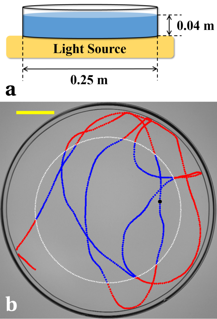
Figure 1: a) Schematic of the experimental setup. b) Trajectory for a single camphoric acid boat. The region within the white dotted line denoting the trajectory in blue is considered for all analysis. The trajectory marked in red is discarded from analysis to avoid systematic errors arising from boundary effects.

Figure 1a shows a schematic of the experimental setup. All experiments were performed in a glass petri dish (0.25 m in diameter) filled with de-ionized water to a height of 0.04 m. A camphoric acid tablet (c-boat) was gently introduced at the air-water interface and its self-motion was recorded with a Nikon D800E camera at 30 frames per second. The petri dish was placed atop a uniform backlit LED illumination source intentionally chosen to operate with direct current to circumvent alternating current flicker in images interfering with post-processing.  The c-boat appears as a dark disk moving in a bright background in this imaging method as shown in figure 1b. The experimental images were post processed with image analysis algorithms written in-house to obtain the c-boat position and velocity as a function of time. The c-boat position and velocity information employed in the analysis was confined to a region 0.036 m away from the walls to exclude boundary effects. Parts of the c-boat trajectory (red in figure 1b) lying outside the dashed white circle in figure 1b at a distance of 0.036 m from petri dish wall were not employed in our analysis in order to exclude boundary effects. This 0.036 m exclusion distance was empirically determined from the longest radial distance over which marangoni spreading of camphoric acid was prominent. Only blue sections of the c-boat trajectory within the inner circle bounded by white dashed line in figure 1b were used in all the analysis.

The shape and size of a chemical-laden tablet, e.g. a camphoric acid tablet, changes over the duration of the experiment as the substance undergoes dissolution or sublimation into the surrounding fluids. To decouple the shape from the chemical composition, the c-boats were constructed by infusing camphoric acid in agarose gel.

The c-boat motion being governed by Marangoni force, surface tension difference between the ambient surface and CA entering the surface forms the primary parameter for this study. Since the c-boat holds a finite quantity of CA, its concentration monotonically decreases with time, thereby continually reducing the strength of the marangoni effect. Independent experiments modifying the ambient surface tension confirmed the role of surface tension difference as the primary parameter. We varied the surface tension of the ambient interface by introducing metered dosage of Sodium Dodecyl Sulfate (SDS) (Wako Pure Chemical Industries, Ltd., Cat. No. 196-08675) from known published tables. Actual surface tension values were also independently confirmed with the pendant drop method on a tensiometer (OneAttension Theta tensiometer).

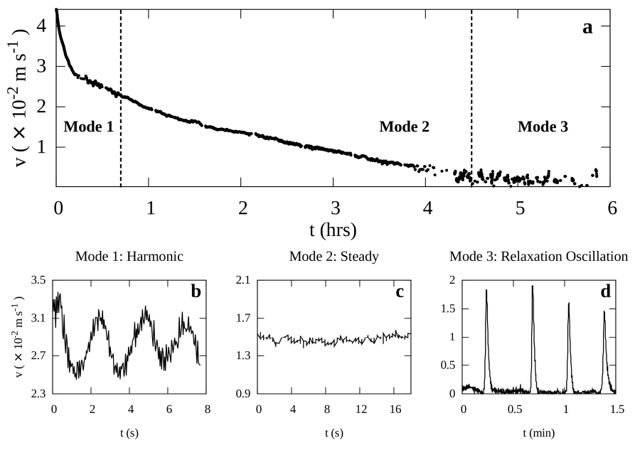
Figure 2: a) Average speed exhibits a monotonic decay with time as the total quantity of camphoric acid within the tablet decreases, thus leading to a reduction in the Marangoni stress. With decreasing average speed, three distinct modes of motion are observed: b) Harmonic mode with sinusoidal oscillations, c) Steady State Mode where the speed is constant modulo fluctuations and d) Relaxation oscillation mode where the camphoric acid boat is static for long durations before jumping to a new location at regular intervals.

 

A moving c-boat leaves camphoric acid in it's wake which can be qualitatively visualised via the distribution pattern of tracer particles decorating the surface figure 3. Hollow silica glass spheres (specific gravity 0.25 and 50 micron diameter) sprinkled onto the air-water interface were used to follow the well defined comet-shaped particle-free region in the wake of a c-boat. The shape of this region provides a qualitative measure of the strength of marangoni force acting on the c-boat.

When a c-boat is placed at the air-water interface, CA spreads radially and sets up axisymmetric interfacial tension gradients around the c-boat. Ambient fluctuations spontaneously break this symmetry and sharpen the gradients along a preferential direction; as a consequence a net force acts on the c-boat and propels it. The boat's motion amplifies the asymmetry and maintains it, thereby permitting it's continued motion. Owing to constant CA dissolution from the interface into the bulk fluid, the c-boat motion continues until it exhausts all CA molecules. With decreasing marangoni force strength in time, the c-boat exhibits three distinct modes of motion.  Figure 2b-d show time traces of instantaneous c-boat speed at specific intervals corresponding to these three modes. At early times and high surface tension difference, the c-boat speed exhibits harmonic oscillations about the mean (see figure 2b). This mean speed and oscillation frequency continuously decrease with time, whereas the oscillation amplitude passes through a maximum before it decreases and transitions to the second distinct mode where the c-boat moves with steady speed (see figure 2c). The third distinct mode of relaxation oscillations emerges at long times and low surface tension differences where c-boat motion occurs in periodic bursts interspersed with durations of almost no c-boat motion (see figure 2d).

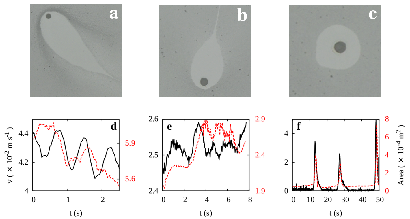
Figure 3: Visualization of the camphoric acid spreading over the surface around a moving camphoric acid boat with tracer particles for (a) Harmonic mode, (b) Steady state mode, and (c) Relaxation oscillation mode. The brighter, tracer-free region has an area that exhibits same behavior as the speed as observed for (d) Harmonic mode, (e) Steady state mode and (f) Relaxation oscillation mode provides experimental evidence in support of the assertion that the modes of motion are a result of Marangoni stress.

 

The continuity of the Marangoni force strength with time can be confirmed via visualization of the comet trail left behind the c-boat. In particular, the comet trail provides a visualization of the asymmetry in the CA distribution around the c-boat. The shape and size of the comet trail is, therefore, indicative of the nature of underlying dynamics. Direct visualization of the comet trail using tracer particles for the three modes of c-boat motion is shown in figure 3a-c. The reducing area of the comet trail suggests a decrease in the net marangoni force strength propelling the c-boat. The elliptical, comet shaped tracer free region in the harmonic mode (figure 3d) gives way to a nearly circular comet shape with a thin wispy tail in the steady mode (figure 3e). The relaxation oscillation mode results in a stationary c-boat with a circular region that grows with time, until a sudden jump in c-boat position results in a momentary comet shape before the c-boat once again settles into a stationary position with a growing circular area (figure 3f).

 

4. Publications

4.1 Journals

Das, T., Lookman, T., & Bandi, M. M. (2015). A minimal description of morphological hierarchy in two-dimensional aggregates. Soft Matter, 11, 6740. doi:10.1039/C5SM01222H

Iikawa, N., Bandi, M. M., & Katsuragi, H. (2015). Structural evolution of a granular pack under manual tapping. Journal of the Physical Society of Japan, 84, 094401.  Retrieved from http://journals.jps.jp/doi/10.7566/JPSJ.84.094401

Savin, T., Bandi, M. M., & Mahadevan, L. (2015). Pressure-driven occlusive flow of a confined red blood cell. Soft Matter, 562-573. doi:10.1039/c5sm01282a

Singh, R. S., Bandi, M., Mahadevan, A., & Mandre, S. (2016). Linear stability analysis for monami in a submerged sea grass bed. Journal of Fluid Mechanics, 786, R1. doi: http://dx.doi.org/10.1017/jfm.2015.642

Bel, G., Connaughton, C., Toots, M., & M., B. M. (2016). Grid-scale fluctuations and forecast error in wind power. New Journal of Physics, 18, 023015. doi:http://dx.doi.org/10.1088/1367-2630/18/2/023015

Iikawa, N., Bandi, M. M., & Katsuragi, H. (2016). Sensitivity of Granular Force Chain Orientation to Disorder-induced Metastable Relaxation. Physical Review Letters, 116, 128001. doi:http://dx.doi.org/10.1103/PhysRevLett.116.128001

4.2 Books and other one-time publications

Nothing to report

4.3 Oral and Poster Presentations

Oral Presentations

Akella, V. S., Singh, D. K., Singh, R. S., Mandre, S., & Bandi, M. M. (2015, 2015.11.23). Hydrodynamics of a self-propelled camphor boat at the air-water interface. Paper presented at the American Physical Society's Division of Fluid Dynamics Annual Meeting, Boston, MA.

Basu, S., Yawar, A., Concha, A., & Bandi, M. M. (2015, 2015.11.22). Modeling drop impacts on inclined flowing soap films. Paper presented at the American Physical Society's Division of Fluid Dynamics Annual Meeting, Boston, MA.

Das, T., Bandi, M. M., & Douglas, J. (2016, 2015.03.17). In search of a corresponding state description of the thermodynamics and dynamics of complex fluids. Paper presented at the American Physical Society's March Meeting 2016, Baltimore, Maryland, USA.

Nguyen, K. D., Yu, N., Bandi, M. M., Venkadesan, M., & Mandre, S. (2016, 2016.03.18). Curvature dependent modulation of fish fin stiffness. Paper presented at the American Physical Society's March Meeting 2016, Baltimore, Maryland, USA.

Singh, D. K., Akella, V. S., Singh, R. S., Mandre, S., & Bandi, M. M. (2015, 2015.11.23). Hydrodynamics of a fixed camphor boat at the air-water interface. Paper presented at the American Physical Society's Division of Fluid Dynamics Annual Meeting, Boston, MA.

Venkadesan, M., Dias, M. A., Singh, D. K., Bandi, M. M., & Mandre, S. (2015, 2015.07.15). Stiffness of the human foot and evolution of the transversal arch. Paper presented at the 15th HFSP Awardees Meeting, La Jolla, CA.

Yawar, A., Basu, S., Concha, A., & Bandi, M. M. (2015, 2015.11.22). Experimental study of drop impacts on soap films. Paper presented at the American Physical Society's Division of Fluid Dynamics Annual Meeting, Boston, MA.

Poster Presentations

Akella, V. S., Singh, D. K., Singh, R. S., Mandre, S., & Bandi, M. M. (2016). Dynamics of self-propelled camphoric acid boat at the air-water interface CompFlu-2016. Pune, India.

Basu, S., Yawar, A., Concha, A., & Bandi, M. M. (2016). Mathematical model for drop impacts on inclined flowing soap films CompFlu 2016. Pune, India.

Mandre, S., Dias, M. A., Singh, D. K., Bandi, M. M., & Venkadesan, M. (2015). How the arches of the feet influence stiffness Dynamic Walking 2015. Ohio State University, Columbus, Ohio.

Seminars

Bandi, M. M. (2015, 2015.5.10). The Spectrum of Wind and Tidal Power Fluctuations OIST Mini Symposium "Small Meets Large: Connecting Microfluidics with Marine Ecology". OIST Main Campus, Seminar Room C209.

Bandi, M. M. (2015, 2015.07.22). The Spectrum of Wind Power Fluctuations. Center for Nonlinear Studies, Los Alamos National Laboratory, Los Alamos, USA.

Bandi, M. M. (2015, 2015.07.27). The Spectrum of Wind Power Fluctuations. Center for Nonlinear Dynamics, University of Texas-Austin, USA.

Bandi, M. M. (2015, 2015.08.07). The Spectrum of Wind Power Fluctuations. Department of Physics, Hong Kong University of Science & Technology, Hong Kong.

Bandi, M. M. (2015, 2015.08.30). The Spectrum of Wind Power Fluctuations. Department of Chemical Physics, Weizmann Institute of Science, Israel.

Bandi, M. M. (2015, 2015.11.19). The Spectrum of Wind Power Fluctuations. James Franck Institute, University of Chicago, Chicago, Illinois, USA.

Bandi, M. M. (2015, 2015.12.02). The Spectrum of Wind Power Fluctuations. Fluids Seminar, School of Engineering, Brown University.

Bandi, M. M. (2015, 2015.12.08). The Spectrum of Wind Power Fluctuations. Physical Mathematics Seminar, Department of Mathematics, Massachusetts Institute of Technology, Cambridge, MA, USA.

Bandi, M. M. (2015, 2015.12.10). The Spectrum of Wind Power Fluctuations. Applied Dynamics Seminar, Department of Physics, University of Maryland, College Park, MD, USA.

Bandi, M. M. (2016, 2016.03.03). The Spectrum of Wind Power Fluctuations. Department of Civil and Environmental Engineering, Stanford University.

Bandi, M. M. (2016, 2016.03.04). The Spectrum of Wind Power Fluctuations. Schlumberger-Doll Research Centre, Cambridge, Massachusetts, USA.

Bandi, M. M. (2016, 2016.03.09). The Spectrum of Wind Power Fluctuations. Department of Mechanical Engineering and Materials Science, Yale University.

5. Intellectual Property Rights and Other Specific Achievements

Nothing to report

 

6. Meetings and Events

6.1 Flapping flexible plate: from caudal fin to submarine propulsor

Date: May 5, 2015

Venue: OIST Campus Lab 2

Speaker: Dr. Florine Paraz (IRPHE & Aix-Marseille University)

 

6.2 Statistical Mechanics of Insect Swarms

Date: June 18, 2015

Venue: OIST Campus Lab 1

Speaker: Prof. Nicholas T. Ouellette (Stanford University)

 

6.3 Information and thermodynamics: Experimental verification of Landauer's erasure principle

Date: Aug 6, 2016

Venue: OIST Campus Lab 3

Speaker: Prof. Sergio Ciliberto (ENS de Lyon)

 

6.4 Tailoring defect densities in crystals using light fields: Amorphization and plastic flow of a solid in a non-affine field

Date: Apr 27, 2016

Venue: OIST Campus Lab 1

Speaker: Prof. Surajit Sengupta (TIFR Centre for Interdisciplinary Sciences)

 

7. Other

Nothing to report.