Complex Fluids and Flows Unit (Marco Edoardo Rosti)

Code - Fujin - Validation - Immersed Boundary Method - Flexible fiber

A hanging filament under gravity

*Sketch of the problem and of the Cartesian coordinate system.*

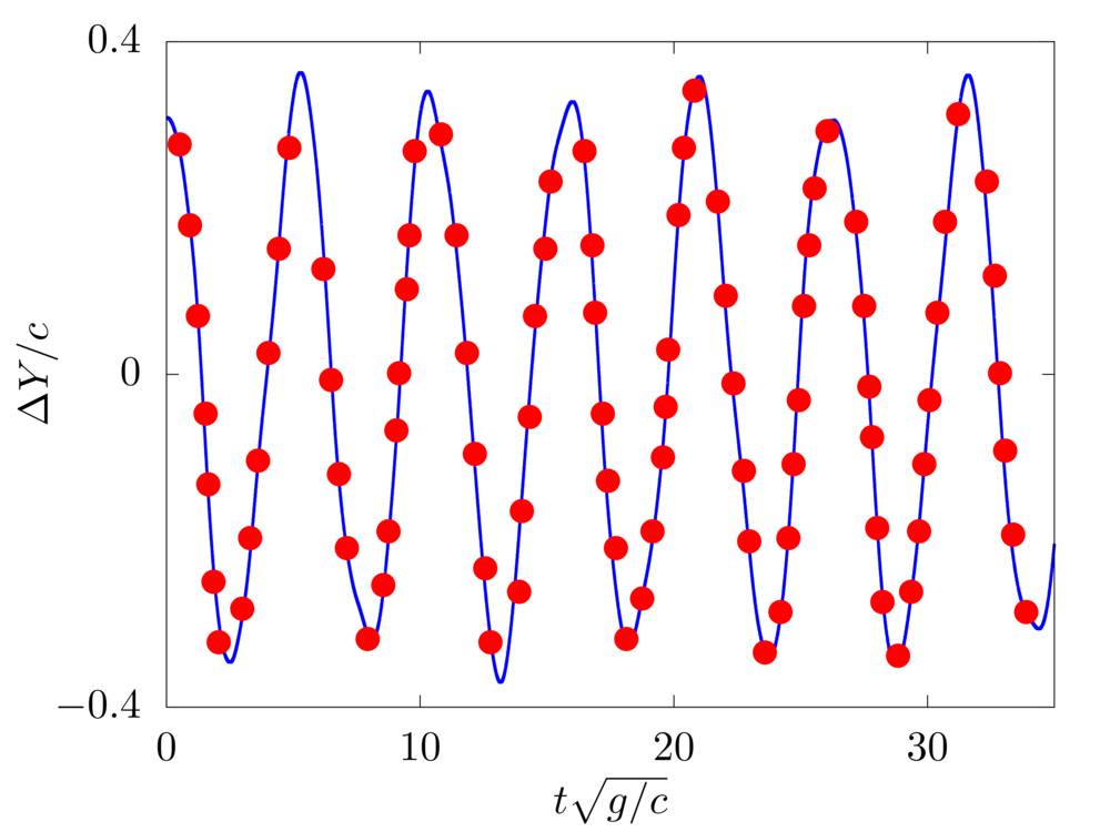
We consider the oscillations of a hanging filament under gravity. A filament of length $c=1m$, linear density difference $\Delta \widetilde{\rho}=1 kg/m$ and flexibility $\gamma=0.01 kg~m^3 / s^2$ is initially held stationary with an angle of $0.1 \pi$ from the vertical and then, after being released, starts swinging due to the gravity force $g=10m/s^2$. The filament is discretised with $100$ Lagrangian points.

config.h

#define _FLOW_CHANNEL_
#define _FLOW_FIXED_
#define _MULTIPHASE_
#define _MULTIPHASE_FIL_
#define _MULTIPHASE_FIL_HING_
#define _MULTIPHASE_FIL_FIXD_

param.f90

! Gravitational acceleration
real, dimension(3), parameter :: gr=(/0.0,10.0,0.0/)
! Number of filaments
integer, parameter :: filN=1
! Number of Lagrangian points per filament
integer, parameter :: filNL=100
! Length of the filaments
real, parameter :: filL = 1.0
! Filament linear density difference and flexibility
real, parameter :: filDRhoL = 1.0, filGamma=0.01

input/input.in

# Simulation initial and final step
0     200000
# Simulation time
0.0
# Simulation time-step
1.0000000000000001E-004
# Output frequency
1     100000       100     1000000      1000000
# Simulation restart condition for the multiphase part
F

*Time evolution of the y-coordinate of the free-end of a filament due to gravity. The line denotes the numerical results and the symbols those from Ref. [1].*

Free vibration of unsupported and cantilevered fibers

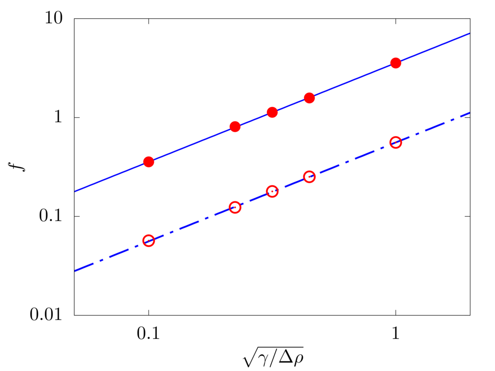
In the absence of any load, we evaulate the free vibration of a fiber. The filament length $c$, flexibility $\gamma$ and linear density difference $\Delta \widetilde{\rho}$ are varied and the resulting frequency $f$ of the free oscillations measured. The filament is discretised with $100$ Lagrangian points.

Analytical solution - free: $f = \frac{22.3733}{2 \pi c^2} \sqrt{\frac{\gamma}{\Delta \widetilde{\rho}}}$ $v (z) = \frac{n}{n + 1} {(\frac{P_{y}}{k})}^{\frac{1}{n}} [h^{\frac{n + 1}{n}} - {(z - h)}^{\frac{n + 1}{n}}]$

Analytical solution - clamped: $f = \frac{3.5161}{2 \pi c^2} \sqrt{\frac{\gamma}{\Delta \widetilde{\rho}}}$

config.h

#define _FLOW_CHANNEL_
#define _FLOW_FIXED_
#define _MULTIPHASE_
#define _MULTIPHASE_FIL_
#define _MULTIPHASE_FIL_FREE_
#define _MULTIPHASE_FIL_FIXD_

param.f90

! Gravitational acceleration
real, dimension(3), parameter :: gr=(/0.0,0.0,0.0/)
! Number of filaments
integer, parameter :: filN=1
! Number of Lagrangian points per filament
integer, parameter :: filNL=100
! Length of the filaments
real, parameter :: filL = 1.0
! Filament linear density difference and flexibility
real, parameter :: filDRhoL = 1.0, filGamma=0.01

input/input.in

# Simulation initial and final step
0     200000
# Simulation time
0.0
# Simulation time-step
1.0000000000000001E-004
# Output frequency
1     100000       100     1000000      1000000
# Simulation restart condition for the multiphase part
F

*Frequency of oscillations of a fiber in void. The solid and dashed lines denote the theoretical results for a free and clamped fiber, while the symbols the numerical results.*

A hanging filament in a uniform flow

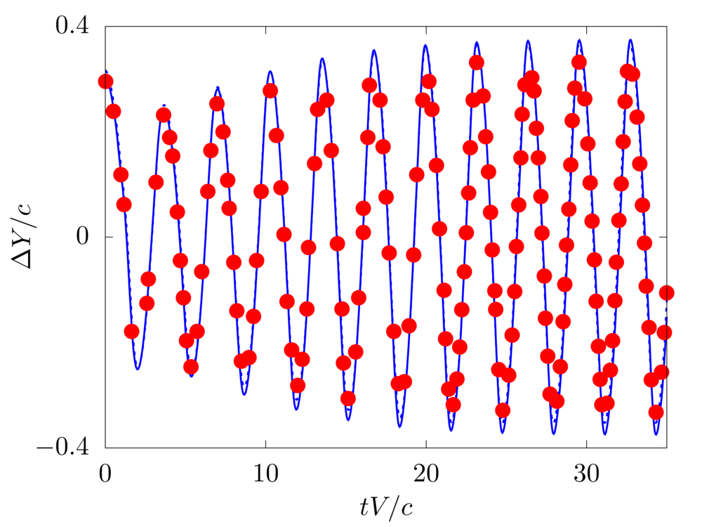
We consider the oscillations of a hanging filament in a uniform flow with velocity $V$. A filament of length $c=1m$, linear density difference $\Delta \widetilde{\rho}=1.5 kg/m$ and flexibility $\gamma=0.0015 kg~m^3 / s^2$ is initially held stationary with an angle of $0.1 \pi$ from the vertical and then, after being released, starts swinging due to the combined effect of the viscous fluid flow ($\nu=0.005m^2/s$) and gravity force ($g=0.5m/s^2$). The filament is discretised with $65$ Lagrangian points.

config.h

#define _FLOW_INOUT_
#define _FLOW_INOUT_UNBOUND_
#define _SOLVER_INOUT_
#define _MULTIPHASE_
#define _MULTIPHASE_IBML_
#define _MULTIPHASE_IBML_GLDS_
#define _MULTIPHASE_IBML_GLDS_2D_
#define _MULTIPHASE_IBML_XXXX_READ_
#define _MULTIPHASE_IBML_XXXX_FIL_
#define _MULTIPHASE_IBML_XXXX_FIL_HING_

param.f90

! Fluid viscosity and density
real, parameter :: vis = 1.0/200.0
real, parameter :: rho = 1.0
! Reference velocity (bulk velocity or wall velocity)
real, parameter :: refVel = 1.0
! Gravitational acceleration
real, dimension(3), parameter :: gr=(/0.0,0.5,0.0/)
! Number of objects
integer, parameter :: ibmlN=1
! Number of Lagrangian points per object
integer, parameter :: ibmlNL=65
! Linear dimension of the object
real, parameter :: ibmlL = 1.0
! Moving or not object
logical, parameter ::  ibmlMoving = .TRUE.
! Filament linear density difference and flexibility
real, parameter :: filDRhoL = 1.5, filGamma=1e-3*filDRhoL

input/input.in

# Simulation initial and final step
0       100000
# Simulation time
0.0
# Simulation time-step
5.0E-004
# Output frequency: 0D, 1D, 2D, 3D, restart data
100       10000        100000     1000000      2000000
# Simulation restart condition for the multiphase part
F

Time evolution of the y-coordinate of the free-end of a filament due to a uniform flow. The line denotes the numerical results and the symbols those from Ref. [1]. The dashed line denotes the numerical results obtained using the RKPM immersed boundary method.

References:

[1] W. X. Huang, S. J. Shin, and H. J. Sung. Simulation of flexible filaments in a uniform flow by the immersed boundary method. Journal of Computational Physics, 226(2):2206–2228, 2007.